Learning Objectives
By the end of this chapter, you should be able to:
Explain the ultraviolet catastrophe and how Planck’s quantization hypothesis resolves it.
State and apply Planck’s radiation law, Wien’s displacement law, and the Stefan–Boltzmann law.
Describe the photoelectric effect and explain why classical (wave) theory fails to account for its observed features.
Apply Einstein’s photon model, , to the photoelectric effect and interpret the stopping-potential and work-function data it predicts.
Explain X-ray production (bremsstrahlung) as an energy-bookkeeping inverse of the photoelectric effect, and apply the Duane–Hunt relation for the minimum X-ray wavelength.
Derive and apply the Compton scattering formula, and explain why Compton scattering demonstrates that photons carry momentum.
Explain pair production and pair annihilation as further evidence for the particle nature of light, and use conservation of energy and momentum to find threshold conditions for each.
Introduction
Chapters 1–3 dismantled the ether and rebuilt kinematics and dynamics on Einstein’s postulates, but light itself — a wave, according to Maxwell’s equations, which special relativity leaves intact — remained conceptually untouched. Chapters 4–5 then developed that wave picture in full quantitative detail: interference and diffraction, both direct, precise confirmations that light obeys a wave equation. This chapter takes up a second, independent crisis of classical physics, one concerning not the kinematics of light but its very nature. Four phenomena — blackbody radiation, the photoelectric effect, X-ray production, and Compton scattering — each show, in a different experimental setting, that electromagnetic radiation exchanges energy with matter not continuously, as a wave should, but in discrete packets. The concept that emerges, the photon, carries energy and momentum , and behaves in each of these experiments like a particle, even though light indisputably also shows the wave behavior of Chapters 4–5 in other settings. A final phenomenon, pair production, shows that a photon’s energy can be converted entirely into matter, tying the particle nature of light directly to the mass–energy equivalence of Chapter 3. Reconciling these two faces of light is the beginning of quantum mechanics.
6.1Blackbody Radiation and Planck’s Hypothesis
Any object at temperature emits electromagnetic radiation across a continuous range of wavelengths, with an intensity distribution depending on . An idealized perfect absorber and emitter is called a blackbody; its emitted spectral distribution, the blackbody spectrum, depends only on temperature, not on the material. A good laboratory approximation is a small hole in the wall of an otherwise closed, heated cavity: radiation entering the hole is absorbed and re-emitted many times by the cavity walls before any of it can escape, so the radiation leaking out through the hole is, to excellent approximation, in thermal equilibrium with the cavity walls and independent of what the walls are made of.
The Ultraviolet Catastrophe
Late-nineteenth-century classical physics attempted to compute this spectrum by treating the electromagnetic field inside the cavity as a superposition of standing-wave modes, each behaving as an independent harmonic oscillator, and invoking the equipartition theorem — every such oscillator, in thermal equilibrium at temperature , should carry average energy , independent of its frequency. Counting the number of standing-wave modes per unit volume in a wavelength interval (a purely geometric problem, fixed by the cavity’s size) and multiplying by per mode gives the Rayleigh–Jeans law,
for the spectral energy density. This matches the observed spectrum reasonably well at long wavelength, but diverges as : since the number of short-wavelength modes grows without bound and each is assigned the same energy , the predicted radiated energy — obtained by integrating over all — is infinite. This absurd prediction, sharply contradicted by the observed spectrum (which rises from zero at short wavelength, peaks, and falls off at long wavelength), became known as the ultraviolet catastrophe: not a small discrepancy to be patched, but a qualitative failure of classical statistical mechanics applied to the electromagnetic field.
Figure 6.1 plots both curves against each other. Raising the temperature moves the peak and lifts the total area, as the next section’s displacement and Stefan–Boltzmann laws require; the classical curve, plotted alongside, runs off the top of the graph at short wavelength no matter what temperature is chosen.
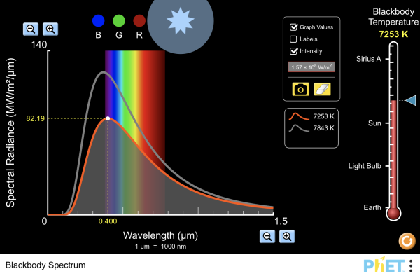
Figure 6.1:The blackbody spectrum as a function of temperature, with the Rayleigh–Jeans prediction available for comparison. The gap between the two at short wavelength is the ultraviolet catastrophe.
Interactive simulation: Blackbody Spectrum
Planck’s Quantization Hypothesis
Max Planck resolved this in 1900 by a hypothesis with no classical justification: the oscillators making up the cavity walls cannot exchange energy with the field continuously, but only in discrete multiples of a fundamental quantum,
where is the oscillator’s frequency and is a new fundamental constant (Planck’s constant), . With this assumption, the average energy of a mode at frequency in thermal equilibrium at temperature is not (the equipartition value, independent of , which causes the catastrophe) but
which suppresses high-frequency (short-wavelength) modes because at high , makes a single quantum too “expensive” to be thermally excited: the Boltzmann factor governing how likely a mode is to hold even one quantum falls off exponentially, cutting off the ultraviolet divergence entirely. This leads to Planck’s radiation law for the spectral energy density,
which matches the observed blackbody spectrum at all wavelengths and temperatures, and reduces to the Rayleigh–Jeans law in the limit , i.e. at long wavelength, where and quantization effects become negligible — exactly the regime in which the classical calculation had already succeeded. Planck himself regarded the quantization of oscillator energy as a mathematical device rather than a physical claim about light. It was Einstein who, five years later, proposed taking it literally.
Wien’s Displacement Law and the Stefan–Boltzmann Law
Differentiating with respect to and setting the result to zero gives Wien’s displacement law for the wavelength of peak emission,
which is why hotter objects glow at shorter (bluer) wavelengths — from the deep red of a heating element to the blue-white of a hot star. Integrating over all wavelengths gives the total power radiated per unit surface area of an ideal blackbody, the Stefan–Boltzmann law,
with the Stefan–Boltzmann constant. The steep dependence means that radiated power is extremely sensitive to temperature: doubling an object’s absolute temperature increases its radiated power per unit area sixteenfold. Real objects are not perfect blackbodies; a surface’s actual radiated power is , where the emissivity measures how closely the surface approximates an ideal absorber and emitter ( for a true blackbody).
Worked Example: The Sun as a Blackbody
The Sun’s surface (photosphere) has an effective temperature of and radius . Treating it as an ideal blackbody, Wien’s law gives the wavelength of peak emission,
squarely in the green part of the visible spectrum — the Sun’s spectrum actually peaks near the middle of the range of wavelengths the human eye evolved to detect, though scattering in Earth’s atmosphere and the eye’s overall spectral response make sunlight appear white or yellow rather than green. The Stefan–Boltzmann law gives the power radiated per unit area, . Multiplying by the Sun’s surface area, , gives a total radiated power (luminosity)
in close agreement with the Sun’s independently measured luminosity of — the same figure used in Chapter 3, Problem 6 to estimate the Sun’s rate of mass loss via . That two completely independent lines of physics (blackbody radiation here, and mass–energy equivalence there) connect so tightly to the same measured number is a testament to how well both theories describe the physical world.
Historical Context: Lenard’s Puzzle
Planck’s quantization hypothesis was aimed narrowly at the blackbody spectrum, and Planck himself did not initially believe that light itself came in discrete packets. Evidence pointing in that direction had, in fact, already been gathering independently. In 1902, three years before Einstein’s photon paper, Philipp Lenard studied the photoelectric effect using an arc lamp and a retarding-voltage apparatus much like the one described below, and found — to general puzzlement at the time — that the stopping voltage (and hence the photoelectrons’ maximum kinetic energy) did not increase with the lamp’s intensity, contrary to every expectation from Maxwell’s wave theory of light, in which a more intense wave carries proportionally more energy to whatever absorbs it. Lenard had no explanation; the result simply sat as an unresolved anomaly in the physics literature for three years, alongside blackbody radiation, until Einstein showed that both puzzles have the same root cause: light exchanges energy with matter in discrete quanta, not continuously.
6.2The Photoelectric Effect and X-Ray Production
The Photoelectric Effect
When light of sufficiently short wavelength strikes a metal surface, electrons are ejected — the photoelectric effect. A typical apparatus measures the photocurrent as a function of a retarding voltage applied between the emitting surface and a collector; the voltage at which the current just reaches zero, the stopping potential , gives the maximum kinetic energy of the ejected electrons, . Plotting the measured photocurrent against retarding voltage traces out a curve that falls smoothly to zero at rather than dropping abruptly, because the ejected electrons are emitted with a distribution of kinetic energies up to , not a single sharp value; marks where even the fastest electrons are turned back.
Three experimental features of this effect resist any explanation in terms of classical electromagnetic waves, in which energy is delivered continuously and is proportional to intensity:
is independent of light intensity. Classically, a more intense wave delivers more energy per unit time to an electron and should eject electrons with more kinetic energy. Experimentally, increasing intensity increases the number of photoelectrons (the current) but not .
depends linearly on frequency, and there exists a sharp threshold frequency , characteristic of the metal, below which no photoelectrons are emitted at all, regardless of intensity or exposure time. Classically, a wave of any frequency should eventually eject electrons if given enough time to deliver sufficient energy, so a hard threshold — and one depending on frequency rather than intensity — has no classical explanation.
Emission is (essentially) instantaneous, with no observable time lag even at very low intensity. Classically, a dim wave should take a measurable time to deliver enough energy to an electron to free it; a rough classical estimate for a very weak source predicts delays of minutes to hours, yet no such delay is ever observed.
Einstein resolved all three in 1905 by proposing that light itself is quantized: it consists of discrete packets, photons, each carrying energy
with the same constant Planck introduced. In the photoelectric effect, a single photon transfers its entire energy to a single electron in one interaction. If (the metal’s work function) is the minimum energy needed to remove an electron from the metal, conservation of energy gives
the photoelectric equation. This immediately explains all three observations: depends on (through the photon energy ) but not on intensity, since intensity only changes the number of photons per second, not the energy of each one; the threshold frequency is , below which a single photon simply does not carry enough energy to free an electron, no matter how many photons arrive; and emission is instantaneous because each electron absorbs one photon’s energy all at once, not gradually. A plot of (equivalently, ) versus is a straight line of slope and -intercept , and Millikan’s precise measurement of exactly this line (1916) provided both a direct experimental value of and strong confirmation of Einstein’s photon hypothesis — for which, not for relativity, Einstein received the 1921 Nobel Prize in Physics.
The three stubborn facts are best met in the order Lenard and Millikan met them, with the apparatus in front of you. In Figure 6.2 the light’s intensity, its wavelength, the target metal, and the retarding voltage are all under control, and the photocurrent and stopping potential are read off directly. Turn the intensity up at fixed wavelength: the current rises and the stopping potential does not move. Shorten the wavelength instead: the stopping potential climbs, and a plot of against — the simulation will accumulate one for you — is a straight line whose slope is and whose intercept names the metal. Cross the threshold from the long-wavelength side and the current stops altogether, at full intensity.
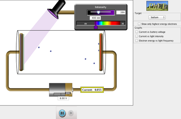
Figure 6.2:The photoelectric apparatus: a photocathode, an adjustable light source, and a retarding voltage. (This is one of PhET’s original Java simulations, run in the browser by CheerpJ; it downloads a Java runtime before it starts, so give it a few seconds on first load.)
Interactive simulation: Photoelectric Effect
Worked Example: The Photoelectric Effect in Cesium
Cesium has one of the lowest work functions of any metal, , which is why it is used in the photocathodes of photomultiplier tubes and early photoelectric light meters.
Ultraviolet light of wavelength illuminates a cesium surface. Using the convenient combination ,
The maximum kinetic energy of the photoelectrons is , so the stopping potential is . The threshold wavelength — the longest wavelength that can still eject an electron — follows from :
which falls in the visible (yellow) part of the spectrum. Cesium is therefore photoelectrically sensitive to ordinary visible light, unlike most metals, whose work functions of 4– push their threshold wavelengths into the ultraviolet.
Applications: Photomultipliers and Photovoltaic Cells
The photoelectric effect underlies two technologies central to modern experimental physics and everyday life. A photomultiplier tube exploits a low-work-function photocathode (often a cesium compound, as in the worked example above) to convert a single incoming photon into a single ejected photoelectron, then accelerates that electron into a series of intermediate electrodes (dynodes), each of which is struck hard enough to eject several additional electrons by secondary emission; the resulting cascade, multiplying the electron count by a factor of a few at each of perhaps ten dynode stages, converts the arrival of a single photon into a macroscopic, easily measured current pulse containing millions of electrons. This single-photon sensitivity makes photomultiplier tubes essential wherever extremely faint light must be detected and counted, including the gamma-ray detectors used in PET scanners (discussed later in this chapter) and in nuclear and particle-physics experiments generally.
A closely related but distinct effect, the photovoltaic effect, underlies solar cells: rather than ejecting an electron entirely from the material, an absorbed photon in a semiconductor promotes an electron across the material’s band gap (the semiconductor analog of the work function, examined further in solid-state contexts), and a built-in electric field at a junction between two differently doped semiconductor layers then separates the resulting electron and the vacancy (hole) it leaves behind before they can recombine, driving a current through an external circuit. As in the ordinary photoelectric effect, only photons with energy exceeding a threshold (the band-gap energy) contribute usable electrons, which is why solar-cell efficiency depends sensitively on matching the semiconductor’s band gap to the solar spectrum.
X-Ray Production: Bremsstrahlung
The photoelectric effect converts a photon into an energetic electron; an energetic electron can conversely give up part of its energy as radiation when it is abruptly decelerated in matter. This bremsstrahlung process is the standard laboratory and industrial method of producing X-rays. It is an energy-bookkeeping inverse of the photoelectric effect, not its literal microscopic time reverse (which would involve radiative recombination into a bound state). In an X-ray tube, electrons are accelerated from rest through a large potential difference (typically tens to hundreds of kilovolts) and strike a dense metal target (commonly tungsten). As each electron decelerates within the target — bremsstrahlung, German for “braking radiation” — it radiates part or all of its kinetic energy as one or more photons.
Because an individual electron can, in principle, lose its entire kinetic energy in a single deceleration event (converting essentially all its kinetic energy into one photon), there is a sharply defined maximum photon energy — and correspondingly a minimum wavelength — that the tube can produce, set by
known as the Duane–Hunt limit. Most electrons instead lose their energy gradually over many collisions, radiating photons of smaller energy at each step and producing a continuous spectrum of wavelengths longer than — but no photon in the entire spectrum can have a wavelength shorter than , since no single electron carries more than of kinetic energy to begin with. Superimposed on this continuous bremsstrahlung spectrum are sharp characteristic X-ray lines, produced when an incident electron knocks an inner-shell electron out of a target atom and an outer electron falls down to fill the vacancy, emitting a photon of energy fixed by the target element’s inner-shell energy levels (Moseley’s law for these characteristic energies is developed in Chapter 11). Unlike the continuous bremsstrahlung background, the characteristic lines depend on the target material, not on the accelerating voltage (once is large enough to eject the inner-shell electron in the first place).
Bremsstrahlung is worth separating into its classical and its quantum halves, because only the second is new here. The classical half — that a charge which accelerates radiates, and that the radiation carries energy away — is already in Maxwell’s equations, and Figure 6.3 is that statement on its own: shake a charge and kinks in its field propagate outward at , taking energy with them. Stopping a charge dead is an acceleration like any other, so an electron slamming into a tungsten anode must radiate. What classical physics cannot supply is the sharp edge at : a continuous field theory sets no floor on the wavelength radiated in a single event, and the Duane–Hunt limit exists only because the radiated energy comes in quanta and one electron brings only to spend.
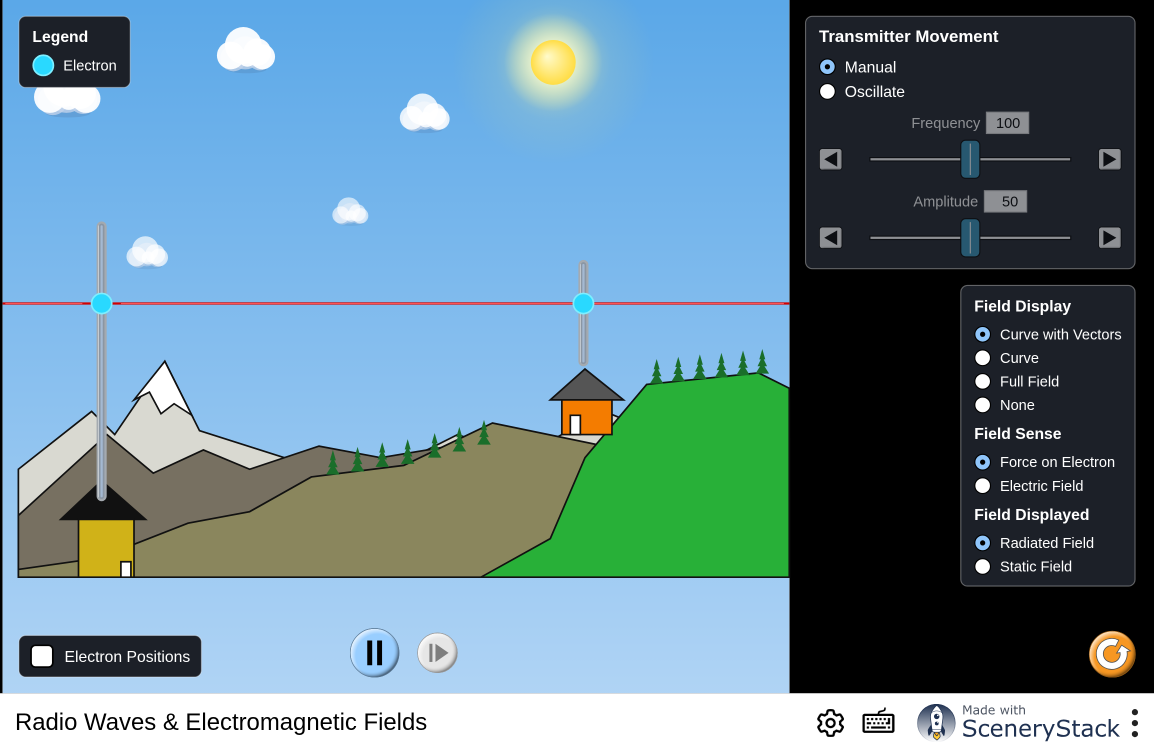
Figure 6.3:An accelerating charge and the field it radiates. Move the charge by hand and watch the disturbance propagate outward at — the classical mechanism behind bremsstrahlung, and the one the electron in an X-ray tube obeys on its way to producing a photon of energy up to .
Interactive simulation: Radio Waves
Worked Example: Minimum Wavelength from a Diagnostic X-Ray Tube
A medical diagnostic X-ray tube is operated at an accelerating voltage of . The Duane–Hunt limit gives
This is comparable to, and somewhat shorter than, typical interatomic spacings in crystals (–), which is why X-rays of this energy scale are useful for crystallographic diffraction (Chapter 5) as well as medical imaging, where their short wavelength (and correspondingly high photon energy) allows them to penetrate soft tissue while being partially absorbed by denser bone.
6.3Compton Scattering, Pair Production, and the Photon
Compton Scattering
Even after the photoelectric effect, one could imagine “photon-like” energy exchange as a property specific to bound electrons in a metal, without light itself consisting of localized particles carrying momentum. Arthur Compton’s 1923 experiment removed this loophole by showing that photons scattering from a free electron transfer momentum exactly as a particle collision would.
In Compton’s experiment, X-rays of a single wavelength are directed at a target of loosely bound (effectively free) electrons, and the wavelength of the scattered X-rays is measured as a function of scattering angle . Classically, an electromagnetic wave incident on a charge should simply drive that charge to oscillate at the incident frequency and re-radiate at the same frequency (Thomson scattering); no wavelength shift is expected. Compton observed a systematic increase in wavelength, , growing with scattering angle and independent of the target material — a signature of a two-body collision, not wave re-radiation.
Deriving the Compton Formula
Treat the photon as a particle with energy and momentum (consistent with the massless-particle limit of the energy–momentum relation from Chapter 3), and apply conservation of relativistic energy and momentum to an elastic collision between the photon and an initially free, stationary electron of mass . Let the photon scatter through angle , emerging with wavelength , while the electron recoils with momentum and (relativistic) energy . The three momentum components entering the collision — incident photon momentum along the initial direction, and zero for the electron — must balance the two outgoing momenta, whose vector sum (photon momentum at angle , electron momentum at some recoil angle) forms a triangle. The law of cosines applied to that triangle gives
Conservation of energy, with the electron initially at rest (), gives
Squaring (ii) and using the energy–momentum invariant from Chapter 3 to eliminate in favor of , then substituting (i) for , produces (after the , , and terms cancel identically between the two sides) the much simpler relation
Dividing through by , multiplying both sides by , and simplifying yields the Compton scattering formula:
The constant is the Compton wavelength of the electron. The formula correctly predicts zero shift at (forward, undeflected “scattering”) and maximum shift at (photon backscattered), matches the observed angular dependence precisely, and — crucially — is independent of the incident wavelength itself, matching experiment. Compton scattering is direct, quantitative confirmation that a photon carries momentum and transfers it to a free electron exactly as one particle colliding with another.
The Compton formula in terms of photon energy
The wavelength form is the natural one for X-ray diffraction work, where wavelengths are measured directly, but gamma-ray spectroscopy — including the Compton-edge discussion below — more often calls for the scattered photon’s energy directly in terms of the incident energy . Substituting and into the Compton formula gives
Multiplying through by and solving for yields
Setting gives the minimum possible scattered-photon energy, , and hence the maximum possible energy that a single Compton-scattering event can deposit in a detector — the location of the Compton edge introduced below.
Worked Example: Compton-Scattered Molybdenum X-Rays
X-rays of wavelength (comparable to characteristic molybdenum X-rays used in crystallography) Compton-scatter off free electrons at . The wavelength shift is
so the scattered wavelength is . In photon-energy terms, the incident photon carries , while the scattered photon carries . The energy transferred to the recoiling electron is therefore — a small but entirely measurable fraction of the incident photon’s energy, exactly the kind of energy loss Compton measured to confirm the formula.
The Compton Edge
In a real gamma-ray or X-ray detector, photons scatter through the full range of angles available inside the detector material, and the detector records the energy actually deposited by the recoiling electron for each scattering event. Because increases monotonically with (least energy transfer for forward scattering, most for backscattering), there is a sharply defined maximum possible energy deposit, occurring at — the Compton edge — beyond which no Compton-scattered electron can deposit more energy in a single scattering event, no matter how many photons are examined. A photon that instead deposits its entire energy in one interaction (via the photoelectric effect on a bound atomic electron, rather than Compton scattering a free one) produces a separate, sharp peak at the full incident photon energy, the photopeak. Gamma-ray spectroscopists routinely distinguish these two features — a sharp photopeak plus a broad continuum of Compton-scattered energies cut off abruptly at the Compton edge — when interpreting a detector’s measured energy spectrum, since both are simultaneous, competing ways the same photon can interact with the detector material.
Pair Production and Annihilation
A further, still more dramatic demonstration of the particle nature of light is pair production: a sufficiently energetic photon, passing near a nucleus, can convert entirely into an electron–positron pair,
requiring a photon energy of at least (twice the electron rest energy) — a direct manifestation of mass–energy equivalence (Chapter 3), converting a massless particle’s energy into the rest mass of two massive particles.
A nearby massive third body — typically an atomic nucleus — is required to conserve momentum. This can be seen directly from the energy–momentum four-vector formalism of Chapter 3: an isolated photon of energy has momentum , but a resulting electron–positron pair with the same total energy (by energy conservation) necessarily has total momentum strictly less than , because each massive particle satisfies , so for each — the pair’s combined momentum cannot match the photon’s original momentum at the same total energy. A nucleus nearby can absorb the small difference in momentum (recoiling with negligible kinetic energy, because its mass is so much larger than ) while barely affecting the energy balance, resolving the mismatch; in a vacuum with no such third body available, momentum conservation alone forbids the process outright, regardless of how much energy the lone photon carries.
The reverse process, pair annihilation, (two photons are required, rather than one, to conserve momentum in the electron–positron center-of-momentum frame — see Chapter 3, Problem 3), converts rest mass entirely back into photon energy and is used, for example, in positron-emission tomography (PET) imaging, where each annihilation of an injected positron-emitting tracer with a nearby atomic electron produces two back-to-back gamma rays that a ring of detectors uses to reconstruct the tracer’s location.
Worked Example: Sharing Energy Above Pair-Production Threshold
A photon of energy , well above the threshold, undergoes pair production near a heavy nucleus. Because the nucleus is far more massive than the electron or positron, it absorbs essentially none of the available kinetic energy (a large mass can supply whatever small momentum balance is needed while carrying away almost no energy, exactly analogous to how a wall barely recoils, and gains almost no kinetic energy, when it reflects a ball). The energy left over after paying the rest-mass cost is therefore shared, to good approximation, between the electron and positron as kinetic energy:
If the pair shares this energy symmetrically (not required by any conservation law, but a useful simplifying assumption), each particle carries about of kinetic energy — comparable to its own rest energy, so each is produced at a substantial fraction of the speed of light.
The Photon: A Unified Picture
Four seemingly unrelated phenomena — blackbody radiation, the photoelectric effect, X-ray production, and Compton scattering — together with pair production and annihilation, are all consequences of a single underlying fact: electromagnetic radiation exchanges energy and momentum with matter in discrete, particle-like quanta, and , rather than continuously. Blackbody radiation shows that an oscillator can only emit or absorb energy in these units; the photoelectric effect shows that a photon transfers its entire energy to a single electron in one step; X-ray production shows how an electron’s kinetic energy can be converted into photons, with a sharply bounded maximum photon energy; Compton scattering shows that a photon carries not just energy but momentum, exchanged with a free electron exactly as in a two-body collision; and pair production and annihilation show that a photon’s energy is, via , interconvertible with the rest mass of matter itself. The characteristic quantum features of all five are explained, quantitatively and without exception, by the same photon concept. Yet, as Chapters 4–5 demonstrated, light also produces interference and diffraction patterns with no possible explanation in a naive particle picture. Chapter 7 confronts this apparent contradiction directly, and shows that it is resolved not by choosing one description over the other, but by recognizing that matter, too, has a wave nature — and that wave and particle descriptions are two complementary faces of a single, more complete quantum picture.
6.4Summary
The blackbody spectrum cannot be explained by the classical Rayleigh–Jeans law, , which diverges at short wavelength (the ultraviolet catastrophe); Planck’s hypothesis that oscillator energy is quantized in units of yields a radiation law matching observation at all wavelengths and reduces to the Rayleigh–Jeans law at long wavelength.
Wien’s displacement law, , and the Stefan–Boltzmann law, , follow from Planck’s radiation law and together determine both the color and total radiated power of a thermal source from its temperature alone.
The photoelectric effect — independent of intensity, a sharp threshold frequency, and instantaneous emission — cannot be explained by classical wave theory but follows directly from Einstein’s photon hypothesis, , via .
X-ray production (bremsstrahlung) is an energy-bookkeeping inverse of the photoelectric effect: decelerating electrons in an X-ray tube produce a continuous spectrum bounded by a sharp minimum wavelength, the Duane–Hunt limit, , since no photon can carry more energy than a single electron’s kinetic energy .
Compton scattering — the angle-dependent wavelength shift of X-rays scattered from free electrons, , derivable directly from conservation of relativistic energy and momentum — shows that photons carry momentum and interact with electrons as particles in an elastic collision.
Pair production (, requiring and a nearby massive body to conserve momentum) and pair annihilation () further confirm that photons are quanta of energy and momentum interconvertible with massive particles.
6.5Problems
Solution to Exercise 6.1 #
Wien’s law gives
The difference from is , or . Therefore, the peak wavelength estimates the solar surface temperature as about , in excellent agreement with the stated value.
Solution to Exercise 6.2 #
Wien’s law gives , which is infrared. The blackbody flux is
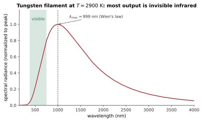
Figure 6.4:The filament’s blackbody curve peaks in the infrared at ; the shaded visible band captures only the small, rising left shoulder of the distribution.
Therefore, the filament peaks near in the infrared and radiates ideally; most of its power is invisible infrared rather than useful visible light.
Solution to Exercise 6.3 #
The radius is . Thus
The ratio is . Therefore, the red giant radiates about , or times the Sun’s luminosity.
Solution to Exercise 6.4 #
Using ,
Since , . At threshold, , so . Therefore, the photon energy is , the largest electron kinetic energy is , the stopping potential is , and the threshold wavelength is .
Solution to Exercise 6.5 #
The frequencies are and . Subtracting for the two data points gives
Then .
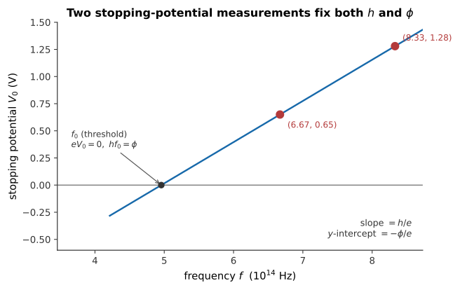
Figure 6.5:The two measurements determine the line completely: its slope gives without assuming a textbook value, and its intercept with gives the threshold frequency .
Therefore, the data give and a work function of .
Solution to Exercise 6.6 #
The incident photon energy is , which exceeds . Thus . The threshold wavelength is
Therefore, ultraviolet light ejects electrons with up to kinetic energy, while visible and near-UV wavelengths longer than cannot overcome platinum’s work function.
Solution to Exercise 6.7 #
An electron accelerated through gains . Hence
Therefore, the minimum wavelength is and the maximum photon energy is ; doubling the voltage halves .
Solution to Exercise 6.8 #
Each incident electron begins with energy , but it can lose any fraction of that energy in one encounter and can lose the rest in subsequent collisions, target excitation, or heat. A photon made in one braking event can therefore have any energy from nearly zero up to , with . Therefore, the many allowed energy shares produce a continuous bremsstrahlung spectrum, even though the endpoint energy and minimum wavelength are sharp.
Solution to Exercise 6.9 #
At , . Thus
The incident energy is , so the electron receives .
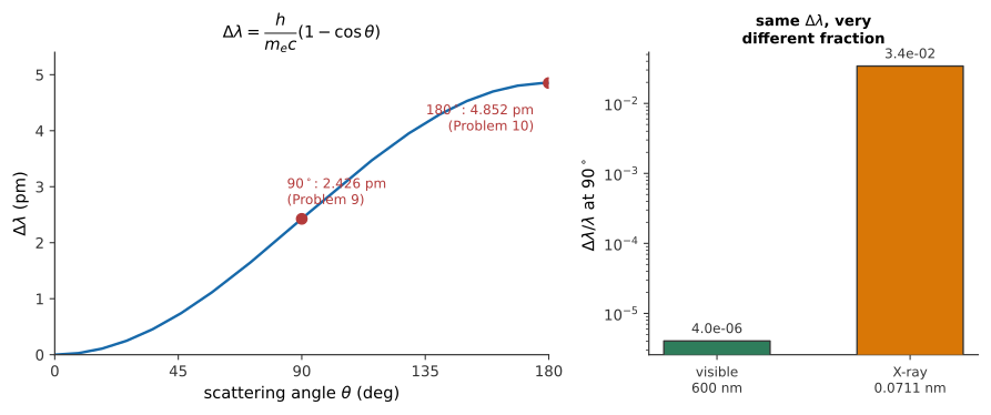
Figure 6.6:Left: depends only on angle, not wavelength; this problem’s shift and Problem 10’s shift are both points on the same curve. Right: the same shift is four parts per million of a visible wavelength but several percent of an X-ray wavelength (Problem 12) — why Compton scattering was discovered with X-rays, not light.
Therefore, the shift is , the scattered photon has wavelength and energy , and the electron receives about .
Solution to Exercise 6.10 #
Putting into gives
For , , so and . This is the endpoint of the same curve shown in Figure 6.6. Therefore, backscattering shifts the wavelength by and transfers nearly of a sufficiently energetic photon’s energy to the electron.
Solution to Exercise 6.11 #
Solution to Exercise 6.12 #
At , . Therefore,
The right-hand panel of Figure 6.6 compares this fraction directly with the X-ray case of Problem 9. Therefore, visible light shifts by only four parts per million, a tiny shift that is difficult to resolve in ordinary Compton-scattering measurements, whereas the same fixed Compton shift is a measurable fraction of an X-ray wavelength.
Solution to Exercise 6.13 #
At minimum, the photon supplies two electron rest energies:
An isolated photon has , but two massive particles with the same total energy have total momentum less than ; energy and momentum cannot both be conserved. Therefore, pair production requires at least photons of wavelength about and a nearby nucleus to absorb recoil momentum.
Solution to Exercise 6.14 #
The rest-energy cost is , leaving
Equal sharing gives and total energy for each.
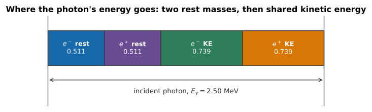
Figure 6.7:The photon’s splits into a fixed entry fee (the two rest masses) and a remaining divided equally as kinetic energy.
Therefore, each particle has kinetic energy and total energy.
Solution to Exercise 6.15 #
At rest the electron and positron have total energy and total momentum zero. The two photons must have equal, opposite momenta and equal energies, so each has . Its wavelength is
Therefore, annihilation produces two opposite gamma rays of wavelength ; a detector ring records their coincident, back-to-back directions to localize the annihilation line through the patient.
Solution to Exercise 6.16 #
The threshold is . Its wavelength is
Compared with the electron-pair threshold wavelength , this is smaller by about 1836, the proton-to-electron mass ratio. Therefore, proton--antiproton production needs about photons with a wavelength.
Solution to Exercise 6.17 #
For scattering, . Hence
Full photoelectric absorption deposits .
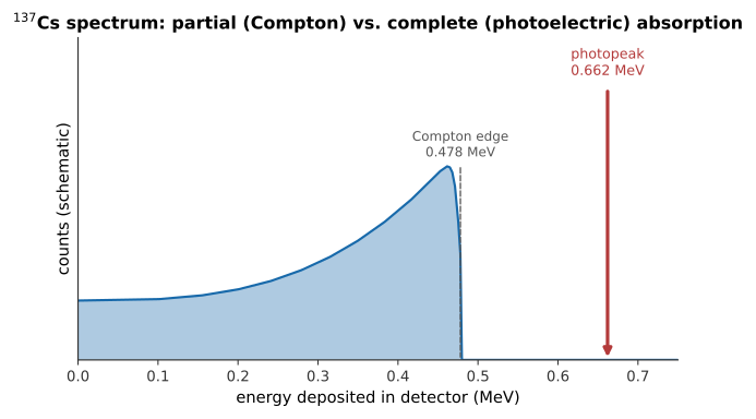
Figure 6.8:A real detector shows both features side by side: a continuum of partial-absorption events ending at the Compton edge, and a separate sharp photopeak from full photoelectric absorption. (Continuum shape is schematic, not the exact Klein–Nishina cross section.)
Therefore, the Compton edge is and the photopeak is ; both appear because photons can either scatter incompletely or be fully absorbed.
Solution to Exercise 6.18 #
The charge needed is , so
Ten stages multiplying by four give electrons, or , below the stated threshold. Therefore, a photomultiplier makes a photon detectable by multiplying one photoelectron into millions, but ten factor-four stages alone are short of a pulse.
Solution to Exercise 6.19 #
Classical treatments assume electromagnetic energy is continuously divisible: cavity modes can receive the continuous equipartition energy , and a brighter wave can transfer energy continuously to an electron. The linked quantum postulates replace this assumption with exchanges in indivisible packets of size : Planck applied the quantization first to the cavity-wall oscillators, suppressing high-frequency modes, and Einstein extended the same quantum of energy to the radiation itself, so one electron receives one photon’s energy at a time. Thus both puzzles share the same cure — energy exchange in units of — even though the photoelectric effect requires the stronger claim that the radiation field itself is quantized.
Solution to Exercise 6.20 #
The threshold condition is , so
This lies in the near infrared. Photon energy above the band gap first creates an electron--hole pair; excess energy is rapidly lost to lattice vibrations rather than producing proportional electrical work. Therefore, silicon can use wavelengths up to about , and photons far above the gap waste much of their extra energy as heat.