Learning Objectives
By the end of this chapter, you should be able to:
Write the time-independent Schrödinger equation in three dimensions and apply it to separable Cartesian potentials such as the 3D infinite box, including cases of partial and full degeneracy.
Explain why central (spherically symmetric) potentials are naturally treated in spherical coordinates, and describe the separation of variables .
Explain the origin and physical meaning of the centrifugal barrier term in the radial equation for a central potential.
Identify the three quantum numbers (, , ) that arise from solving a central-potential problem and state the physical quantity each one labels; for the Coulomb potential, relate the radial quantum number to the principal quantum number .
State the quantization of orbital angular momentum magnitude and -component, and explain the physical meaning of each, including the commutation relations that forbid simultaneous knowledge of more than one Cartesian component.
Describe the isotropic three-dimensional harmonic oscillator as a second exactly solvable central potential and relate its degeneracy structure to the nuclear shell model.
Explain why the three-dimensional treatment is the necessary foundation for the hydrogen atom, developed in Chapter 10.
Introduction
Chapter 8 solved the Schrödinger equation for several one-dimensional potentials, but every atom, molecule, and nucleus is a three-dimensional object, and the most important potential in atomic physics — the Coulomb attraction between an electron and a nucleus — depends only on the distance from a fixed center, not on a single Cartesian coordinate. This chapter extends the Schrödinger equation to three dimensions and develops the machinery — separation of variables in spherical coordinates, the centrifugal barrier in the radial equation, and the angular momentum quantum numbers that emerge from it — needed to solve any central-potential problem, of which the hydrogen atom (Chapter 10) is the most important example. The results obtained here, especially the quantization of angular momentum, apply unchanged to every central potential, not just the Coulomb potential, and reappear throughout atomic, molecular, and nuclear physics.
9.1Three Dimensions and Central Potentials
The Schrödinger Equation in Three Dimensions
Generalizing Chapter 8 to three spatial dimensions, the time-independent Schrödinger equation for a particle of mass in a potential is
or, compactly, , where is the Laplacian operator. As in one dimension, gives the probability of finding the particle in the volume element about , and must be normalizable: .
When the potential is separable in Cartesian coordinates, , the equation can be solved by seeking product solutions , which reduces the problem to three independent one-dimensional Schrödinger equations, one per coordinate, each solved exactly as in Chapter 8. For a 3D infinite box of side lengths (a direct generalization of the infinite square well), this gives
with three independent quantum numbers, one per dimension. A notable feature not seen in one dimension: for a cubic box (), distinct combinations of — e.g., , , — can give the same total energy. This is called degeneracy, and it is a recurring feature of higher-dimensional quantum systems, generally traceable to an underlying symmetry of the potential (here, the equivalence of the three directions in a cube).
Worked Example: A Rectangular Quantum Dot
A semiconductor quantum dot confines an electron in a box with but (a “square” cross-section, but elongated along ) — a shape with less symmetry than a cube, but more than a fully generic box. Using (a convenient rewriting of Equation (9.2) for an electron), the ground state has
a confinement energy of a few tens of millielectronvolts, comparable to at room temperature () — which is why quantum-dot devices are often cooled to enhance the visibility of their discrete energy levels. Because , the box retains a partial symmetry: states and are degenerate for any choice of (swapping the two equal dimensions changes nothing), but states that instead permute the unequal dimension, such as versus , are generally not degenerate with or with each other. A box with would restore full degeneracy among all permutations of a given triple, while a fully generic box () would show no degeneracy at all — the amount of degeneracy is a direct fingerprint of how much geometric symmetry the confining potential actually has.
Central Potentials and Spherical Coordinates
The Coulomb potential, and most potentials of physical interest in atomic and nuclear physics, depend only on the distance from a fixed point: , where . Such a potential is generally not separable in Cartesian coordinates (the isotropic oscillator discussed later is an important exception), but it is separable in spherical coordinates , precisely because its symmetry matches that coordinate system. Written in spherical coordinates, the Schrödinger equation for a central potential admits solutions of the separable form
where , the radial wave function, depends on the specific form of and carries the information about the particle’s radial probability distribution, while , the angular wave function, turns out to be completely independent of the specific form of — it is determined entirely by the requirement that be single-valued and well-behaved on the sphere, and is therefore the same set of functions for the hydrogen atom, a 3D harmonic oscillator, or any other central potential.
Spherical Harmonics: The Lowest Few Explicitly
The angular functions that solve the angular equation are called spherical harmonics, conventionally written and labeled by exactly the two angular quantum numbers introduced below. The lowest few, up to overall normalization constants, are
and already illustrate the general pattern. The harmonic, , is completely independent of and — an -state wave function is spherically symmetric, with a probability density depending only on , the same in every direction from the center. The harmonics depend on angle: , proportional to , is largest along the -axis and vanishes in the -plane (a -type angular distribution, in the language used for atomic orbitals in Chapter 10), while , proportional to , is largest in the -plane and vanishes along the -axis. Each higher introduces additional angular structure — more lobes, more angular nodes — but, crucially, the same three functions describe the angular dependence of a -state electron in hydrogen, a -state neutron in a nuclear shell-model potential, or a -state particle in the isotropic oscillator discussed later in this chapter, since (as already emphasized) the angular equation and its solutions never reference at all.
The Radial Equation and the Centrifugal Barrier
Substituting into the full Schrödinger equation and separating variables reduces the radial part to an ordinary differential equation for . It is standard, and illuminating, to write this in terms of , in which case the radial equation takes a form directly analogous to a one-dimensional Schrödinger equation for on the half-line :
where is the orbital angular momentum quantum number introduced below. The extra term, , is called the centrifugal barrier: it behaves as an additional repulsive potential that grows without bound as (for any ), pushing the particle’s radial probability density away from the origin. This is the quantum-mechanical counterpart of the classical fact that a particle with nonzero angular momentum cannot reach the force center while its angular momentum remains nonzero. For (an s-state, in the spectroscopic notation below), the centrifugal barrier vanishes entirely, and for the usual regular central potentials only states can have a nonvanishing probability density exactly at — a fact used directly in Chapter 10 to explain, for instance, which hydrogen atomic states can undergo processes that require the electron to overlap with the nucleus.
Deriving the Radial Equation for u(r) = rR(r)
Separating in the full Schrödinger equation leaves obeying
with the eigenvalue supplied by the angular equation. The first term mixes a first and second derivative of , which is exactly what the substitution , i.e. , is designed to clean up:
Multiplying the radial equation by and substituting this result gives
exactly the one-dimensional-looking form quoted in the main text. The simplification comes with a boundary condition: for a usual regular central potential, physical regularity requires to stay finite as , and hence — playing the same role here that plays at the rigid wall of a one-dimensional infinite well.
9.2Orbital Angular Momentum
The separation above is not a mathematical accident: it reflects the fact that a central potential exerts no torque about the force center (the force is always radial), so orbital angular momentum, , is conserved, exactly as in classical central-force motion (e.g., Kepler orbits). Solving the angular equation subject to the single-valuedness of shows that the magnitude and one Cartesian component (conventionally the -component) of are simultaneously quantized:
where is the orbital angular momentum quantum number and is the magnetic quantum number, so named because determines how the system’s energy shifts in an external magnetic field (Chapter 11). For a given , there are allowed values of , corresponding to distinct orientations of the angular momentum vector relative to the chosen -axis — a specific, testable manifestation of space quantization: the orbital angular momentum vector does not merely have a quantized length, it can only point in a discrete set of directions relative to an external axis, rather than any direction whatsoever as classical mechanics would allow.
Two features are worth emphasizing, since both run against classical intuition. First, , not — the “extra” factor means that for any the angular momentum vector’s length is slightly larger than its maximum possible -component, ; the vector can never point exactly along the -axis. Second, because and are not simultaneously measurable with , only the magnitude and a single component can be assigned definite values at once — the other two components remain fundamentally indeterminate, consistent with the vector never lying exactly along any single axis.
Historically, states of a given are labeled by spectroscopic letters inherited from early atomic spectroscopy: are denoted respectively — a labeling convention used throughout atomic physics (Chapters 10–11) and retained today purely by tradition.
Why Is Called the Magnetic Quantum Number
The name “magnetic quantum number” is not arbitrary bookkeeping. A charged particle with orbital angular momentum circulating about a center behaves, classically and quantum mechanically alike, as a tiny current loop with an associated orbital magnetic dipole moment,
for an electron of charge , directed opposite to because the electron’s charge is negative. Placed in an external magnetic field along the -axis, this moment contributes an additional term to the electron’s energy, , proportional directly to the magnetic quantum number: each of the otherwise energy-degenerate orientations of acquires a distinct energy shift once a magnetic field is applied, splitting a single spectral line into closely spaced components. This splitting — the (normal) Zeeman effect — was observed spectroscopically well before quantum mechanics existed and is precisely why earned its name: it is the quantum number that controls how atomic energy levels respond to an external magnetic field, a connection developed quantitatively in Chapter 10 and Chapter 11, alongside the further complication (electron spin) required to explain the full richness of observed atomic spectra in a magnetic field.
That a magnetic field sorts a beam into a discrete number of orientations — rather than the continuum a classical dipole would give — is the content of Figure 9.1. Firing spin- atoms through a single analyzer splits the beam in two; chaining analyzers at different angles shows that the measurement does not simply read a pre-existing orientation.
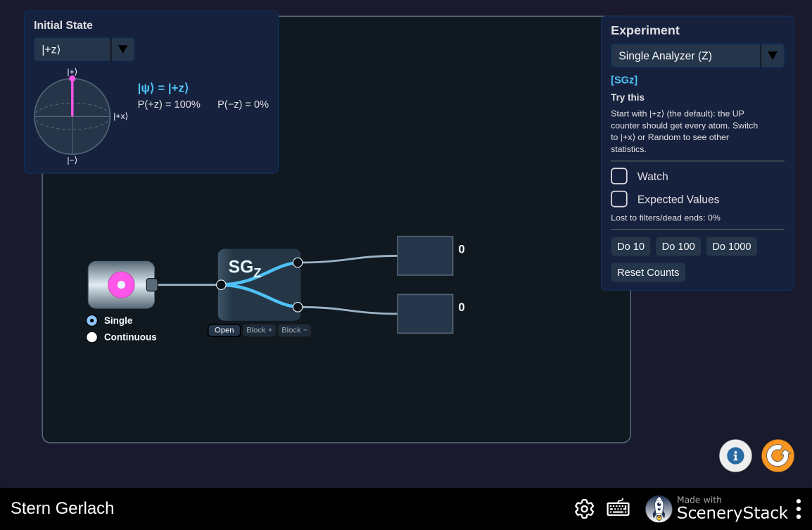
Figure 9.1:The Stern–Gerlach experiment, assembled from analyzers, magnets, and counters. Monte Carlo counts accumulate alongside the analytic quantum prediction, so the (or, for spin, ) discrete outcomes can be checked against the statistics.
Interactive simulation: Stern Gerlach
Worked Example: The Vector Model for 
An electron is in a state with orbital angular momentum quantum number (a -state). Its angular momentum magnitude is
while the maximum possible -component is . The smallest possible angle between and the -axis, achieved when takes its largest value, is
confirming explicitly that can never point exactly along (which would require ) no matter how large is chosen for a given ; the discrepancy versus shrinks only in a relative sense as grows large, another instance of the correspondence principle encountered in Chapter 8.
The cone that this worked example describes is usually drawn as a static picture, which makes the indeterminacy of and look like an admission of ignorance about a vector that is really sitting still somewhere on the cone. The classical system that gets the geometry right is a gyroscope, Figure 9.2: gravity applies a torque perpendicular to the spin angular momentum, and the response is not to tip the axis over but to walk it around a cone at fixed polar angle, with and both constant while and oscillate. Put a magnetic moment in a field instead of a top in gravity and the equation of motion is the same one; the quantum content is only that the cone’s opening angle may take just values.
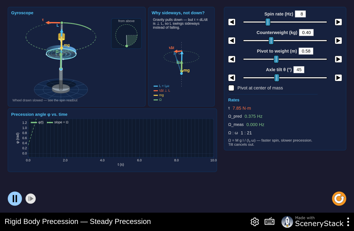
Figure 9.2:A spinning top under gravity. In steady precession the torque stays perpendicular to , so it changes the direction of the angular momentum without changing either its magnitude or its vertical component — the classical motion behind the vector model’s cone, and behind the Larmor precession of a magnetic moment in a field (Chapter 10).
Interactive simulation: Precession
Angular Momentum Commutation Relations
The impossibility of simultaneously sharp values for more than one Cartesian component of is not merely observed; it follows from the algebra of the angular momentum operators themselves, which satisfy the commutation relations
(a cyclic pattern in ), together with . Two operators that do not commute cannot, in general, have simultaneous eigenstates — precisely the mathematical statement of the uncertainty principle applied to angular momentum, directly analogous to the position–momentum commutator underlying the Heisenberg relation of Chapter 7. Because commutes with (and likewise with and ), a quantum state can be prepared with simultaneously sharp values of and one chosen component — exactly the states labeled by and above — but, for , never with sharp values of , , and all at once.
9.3Quantum Numbers and the Isotropic Oscillator
The Three Quantum Numbers of a Central-Potential Bound State
Solving the full three-dimensional problem for a bound state in a central potential produces three quantum numbers, each arising from a separate boundary condition in the separation of variables:
, the radial quantum number, , counting the radial nodes and arising from solving the radial equation subject to normalizability. The energy generally depends on both and ; for the Coulomb potential it is convenient to replace and by the principal quantum number , as shown in Chapter 10;
, the orbital angular momentum quantum number, , governing the magnitude of orbital angular momentum;
, the magnetic quantum number, , governing the orientation of orbital angular momentum relative to a chosen axis.
This trio of labels, with the same angular ranges and physical meanings, appears in every central-potential problem in this book — it is a consequence of three-dimensional rotational symmetry, not a special feature of any one potential. Only the Coulomb problem promotes the combination to a principal quantum number whose energy is independent of ; Chapter 10 specializes the general machinery to that case.
A Second Exactly Solvable Central Potential: The Isotropic Harmonic Oscillator
The Coulomb potential of Chapter 10 is the most important central potential in atomic physics, but it is not the only one that can be solved exactly. The isotropic three-dimensional harmonic oscillator, , is a second example, and it is central (in the technical sense of depending only on ) even though it is also separable in Cartesian coordinates, since splits into three independent one-dimensional oscillators. Solved in Cartesian form, using the one-dimensional harmonic-oscillator result of Chapter 8 three times over, the energy levels are
depending only on the sum , not on how it is distributed among , , individually. The isotropic oscillator has continuous rotational symmetry, which guarantees the degeneracy of each angular-momentum multiplet; its larger degeneracy across different values at fixed reflects an additional oscillator symmetry. The same energy levels can equally well be labeled, via the spherical-coordinate separation of this chapter, by a radial quantum number and , with ; the two labeling schemes describe the same physical states, related by a change of basis, and the total degeneracy of a given level works out to .
This may look like a mathematical curiosity, but the isotropic harmonic oscillator is directly useful: it is the starting point for the nuclear shell model (Chapter 13), in which each nucleon moves, to a first approximation, in an average central potential produced by all the other nucleons — a potential that resembles a finite well but is often approximated, for the purpose of a first, analytically tractable calculation, by an isotropic harmonic oscillator. The oscillator’s degenerate energy levels, once a spin-orbit correction (introduced in Chapter 13) is added, reproduce the empirically observed nuclear magic numbers — proton or neutron counts (2, 8, 20, 28, 50, 82, 126) at which nuclei are unusually stable — in much the same way that filled electron shells explain the chemical stability of the noble gases (Chapter 11).
Comparing Degeneracy Across Three Central Potentials
It is worth pausing to compare the degeneracy patterns of the three central (or Cartesian-separable) potentials encountered so far, since the comparison sharpens exactly what “degeneracy reflects underlying symmetry” means in practice. The cubic infinite box has a discrete symmetry (the box is invariant only under swapping , , and reflections, not under arbitrary rotations), and correspondingly modest degeneracies, arising only from specific numerical coincidences among sums of squares of integers. The isotropic harmonic oscillator has full continuous rotational symmetry plus an additional symmetry responsible for its larger degeneracy across different values at fixed . The hydrogen atom’s Coulomb potential (Chapter 10) has an additional degeneracy as well: not only is the energy independent of (true for any central potential, since no central potential singles out a preferred direction in space), but for the Coulomb potential specifically, the energy is also independent of for fixed principal — an extra, “accidental” degeneracy not explained by rotational symmetry alone, and one of the most distinctive mathematical features of the potential, examined further in Chapter 10.
9.4Summary
The 3D Schrödinger equation, , reduces to three independent 1D equations for a Cartesian-separable potential (e.g., the 3D infinite box), which can produce degeneracy — distinct quantum states sharing the same energy — as a signature of underlying symmetry; a box with partial symmetry (e.g., a square cross-section but different height) shows partial degeneracy, while a fully generic box shows none.
A central potential, , is separable in spherical coordinates as ; the angular part is universal, independent of the specific form of , while the radial equation for contains a repulsive centrifugal barrier term that vanishes only for .
Orbital angular momentum is quantized in both magnitude, (), and -component, () — space quantization — with allowed orientations for each . The commutation relations (and cyclic permutations) show algebraically why and remain simultaneously indeterminate once and are sharp.
The spherical harmonics are the universal angular wave functions of any central potential; the harmonic is spherically symmetric, while harmonics have the angular shape familiar from -orbitals in Chapter 10.
Three quantum numbers, , , , characterize a bound state in a central potential; for the Coulomb potential, the radial and angular labels are often reorganized as , , . States are conventionally labeled for . The magnetic quantum number controls how a state’s energy shifts in an external magnetic field (the Zeeman effect), which is the origin of its name.
The isotropic 3D harmonic oscillator, , is a second exactly solvable central potential, with energies depending only on and highly degenerate levels — the starting point for the nuclear shell model of Chapter 13.
9.5Problems
Solution to Exercise 9.1 #
The box energy in the stated unit is . The three lowest distinct values are 3 from (degeneracy 1), 6 from permutations of (degeneracy 3), and 9 from permutations of (degeneracy 3). Therefore, the first three energy levels are 3, 6, and 9 times , with degeneracies 1, 3, and 3.
Solution to Exercise 9.2 #
Using ,
Interchanging and changes nothing, but this state already has ; permutations involving change the energy because . Therefore, has energy and no distinct symmetry partner at that energy.
Solution to Exercise 9.3 #
For , . The magnitude is , while the largest component is . Since , the vector retains an unavoidable transverse component, as drawn in Figure 9.3.
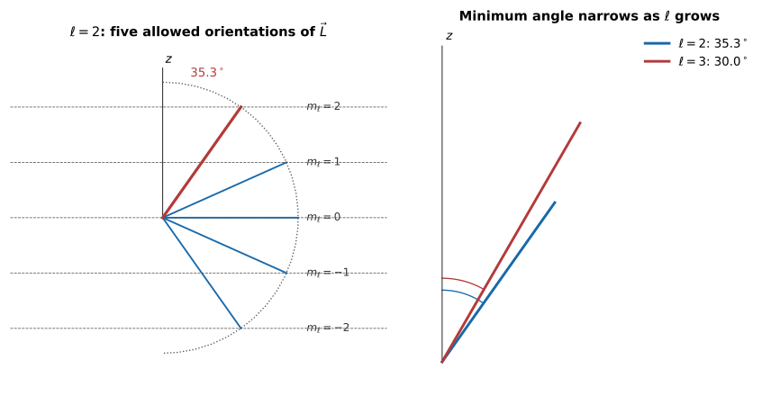
Figure 9.3:Left: the five allowed orientations of for ; even the steepest one, , sits off the -axis. Right: Problem 9’s comparison — the minimum angle shrinks to for , as grows faster than its maximum projection .
Therefore, the allowed values are -2 through +2, and even the largest is strictly less than .
Solution to Exercise 9.4 #
For a Coulomb bound state with , . The combinations are ; ; and . Their total is . Therefore, there are nine allowed states in the shell.
Solution to Exercise 9.5 #
Because is generally nonzero, exact values of and cannot be simultaneous observables. A state with definite and therefore has uncertain transverse components, so its angular-momentum vector cannot lie exactly along the axis unless . Therefore, component uncertainty is precisely why orbital angular momentum is represented by a cone rather than a fixed vector direction.
Solution to Exercise 9.6 #
For a Coulomb state with , can be , so the maximum is . The total number is . Therefore, the shell permits maximum orbital quantum number 3 and contains sixteen states.
Solution to Exercise 9.7 #
When the Schrödinger equation separates, every angular derivative occurs in the angular equation and fixes the spherical harmonics . The potential appears only in the radial equation. Therefore, all central potentials share the same angular functions, while their radial functions and energies differ.
Solution to Exercise 9.8 #
For , the centrifugal term is zero, so there is no angular-momentum barrier at . For , it diverges positively as , suppressing the wave function near the nucleus.
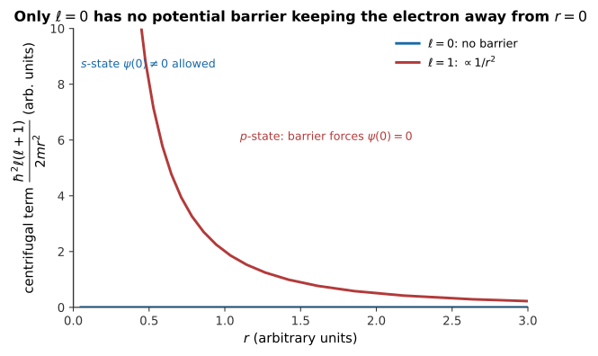
Figure 9.4:For the centrifugal term is identically zero, so nothing prevents ; for it diverges as , an infinitely steep repulsive wall that forces .
Therefore, electrons can penetrate to the nucleus whereas electrons cannot.
Solution to Exercise 9.9 #
The smallest angle occurs for :
For , and , both shown together in Figure 9.3. Therefore, an state reaches , closer to the axis than a state; the cone narrows as increases.
Solution to Exercise 9.10 #
Cycling gives and then , consistent with the stated relation. In contrast, for each component . Therefore, commuting of with one Cartesian component guarantees that and one chosen component can be simultaneously sharp.
Solution to Exercise 9.11 #
The nonnegative triples summing to 2 are . There are six, and the formula gives . Figure 9.5 carries this same degeneracy count into Problem 13’s nuclear-shell application. Therefore, the oscillator shell has exactly six spatial states.
Solution to Exercise 9.12 #
The cubic box has only discrete rotational/permutation symmetry, and its energy depends on the separate squares . The isotropic oscillator has continuous rotational symmetry and energy depending only on the sum , so many more partitions share one energy. Therefore, the oscillator’s larger symmetry produces its larger degeneracy.
Solution to Exercise 9.13 #
The spatial degeneracies are 1, 3, and 6 for . Including spin gives shell capacities 2, 6, and 12, so cumulative capacities are 2, 8, and 20.
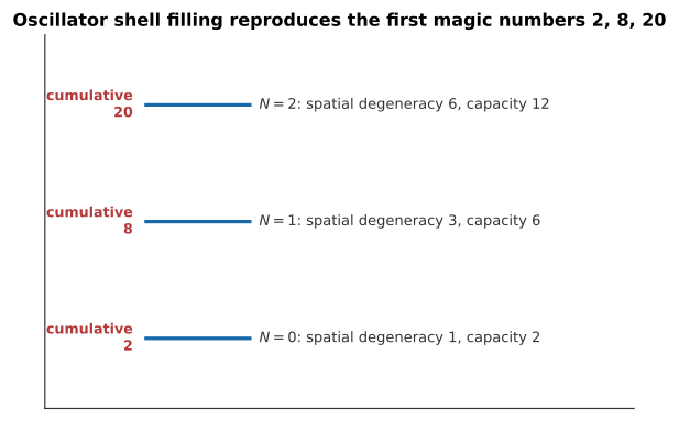
Figure 9.5:Filling the oscillator shells in order, the running total after each shell — 2, 8, 20 — lands exactly on the first three nuclear magic numbers.
Therefore, the simple oscillator model reproduces the first three nuclear magic numbers 2, 8, and 20 before spin--orbit corrections are needed.
Solution to Exercise 9.14 #
For the Coulomb shell, the states are and . The maximum is therefore obtained for , . Then and , so . Therefore, the maximum-projection state has , , and a angle to .
Solution to Exercise 9.15 #
Because , it vanishes where , namely at . This nodal plane leaves two lobes on the positive and negative axes, hence the name .
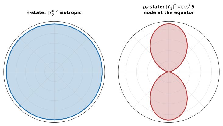
Figure 9.6:The -state angular density is a circle — the same in every direction. The -state density is a dumbbell with a node at , concentrating probability along .
Therefore, is directional with an equatorial node, unlike an state whose angular probability is uniform in every direction.
Solution to Exercise 9.16 #
For , , so a shift proportional to produces three distinct levels. For , only exists and the orbital shift is zero.
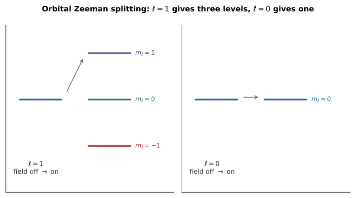
Figure 9.7:Turning on the field splits the level into three, one for each ; the level has only to begin with, so there is nothing to split.
Therefore, a level splits into three orbital Zeeman components while an level does not split orbitally.
Solution to Exercise 9.17 #
Substitution gives
Each independent one-dimensional coordinate contributes . Therefore, the three-dimensional ground state has .
Solution to Exercise 9.18 #
For a general central potential, the radial equation can yield energies that depend separately on the radial and angular quantum numbers, ; then the extra degeneracy among different values found in a Coulomb shell is absent. Coulomb’s potential is special in giving energy depending only on . The isotropic oscillator instead depends on , so it has degeneracy among different combinations but not the Coulomb all- degeneracy at fixed . Therefore, its degeneracy is special but not the same Coulomb accidental degeneracy.
Solution to Exercise 9.19 #
For an electron, and hence . The orbital magnetic moment is then , so there is no orbital force to split the beam. Therefore, silver’s Stern--Gerlach splitting requires electron spin, not orbital angular momentum.