Learning Objectives
By the end of this chapter, you should be able to:
State the time-dependent and time-independent Schrödinger equations and explain the role of each.
Interpret the wave function statistically (the Born interpretation) and apply normalization.
State and apply the boundary and continuity conditions on acceptable wave functions.
Compute expectation values of position and momentum from a wave function using the position and momentum operators.
Solve the time-independent Schrödinger equation for a particle in an infinite square well and interpret the resulting quantized energies and stationary states.
Analyze a potential step and compute reflection and transmission coefficients, and explain why quantum mechanics allows partial reflection even when .
Solve (qualitatively and, for simple cases, quantitatively) the finite square well and explain barrier penetration and quantum tunneling.
Solve the quantum harmonic oscillator, apply its selection rule, and compare its energy spectrum and ground-state behavior to the classical oscillator.
Introduction
Chapter 7 established that a wave packet, not a point trajectory, is the appropriate description of a quantum particle, and that this wave nature is directly responsible for the Heisenberg uncertainty principle. This chapter introduces the equation that governs how such a wave evolves: the Schrödinger equation, proposed by Erwin Schrödinger in 1926. It plays the role in quantum mechanics that Newton’s second law plays in classical mechanics — given a system’s wave function at one instant and the forces (via a potential energy function) acting on it, the Schrödinger equation determines the wave function at all later times. Solving it for a sequence of increasingly realistic potentials — a particle confined to a box, a particle encountering a step or barrier, a particle in a parabolic potential — reveals features with no classical counterpart: quantized energy levels, a nonzero minimum energy, partial reflection where classical physics predicts certain transmission, and the ability of a particle to be found where classical mechanics says it cannot.
8.1The Wave Function and the Schrödinger Equation
The Wave Function and Its Interpretation
Quantum mechanics represents a particle’s state by a complex-valued function of position and time, (in one dimension), called the wave function. Max Born proposed the interpretation now universally adopted: is the probability of finding the particle between and at time , if a position measurement is performed. Because the particle must be found somewhere, an acceptable wave function must be normalized:
For to yield a sensible probability density, it (and, where the potential is finite, its first derivative) must be single-valued, finite, and continuous; discontinuities or divergences in would correspond to ill-defined or infinite probability densities.
The Born rule is easy to state and easy to under-read, because probability is also what a classical physicist reaches for when describing ignorance about a definite fact. The two are not the same, and Figure 8.1 is built around the difference. Its first screen puts a classical coin under a cover beside a quantum one: both give heads half the time, but the classical coin already is heads or tails while it is hidden, and the quantum one is in a superposition of the two until it is looked at. Its later screens make the distinction operational — single photons through a polarizer arriving with probability , and spin- particles through a chain of analyzers whose statistics no assignment of pre-existing values reproduces.
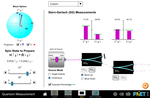
Figure 8.1:Measurement statistics for a classical coin, for single photons through a polarizer, and for spin- particles. is a probability, but not a probability about something already decided — the distinction this chapter’s mathematics quietly assumes.
Interactive simulation: Quantum Measurement
Expectation Values and Operators
Because gives only a probability distribution, not a definite trajectory, a quantum “measurement” of position generally yields different results on identically prepared systems, with a statistical average — the expectation value — defined by
the same weighted-average construction used for any probability distribution in statistics, here weighted by . Momentum, energy, and other physical quantities are represented in quantum mechanics by operators acting on — most importantly the momentum operator , already implicit in the correspondence used to motivate the Schrödinger equation below — and their expectation values follow the same sandwich pattern,
Expectation values are the quantities that connect the abstract wave function to numbers that can be compared with experiment: repeating a position (or momentum) measurement on many identically prepared copies of the same system and averaging the results reproduces (or ), while the statistical spread of those repeated measurements is exactly the (or ) appearing in the Heisenberg uncertainty principle of Chapter 7.
Ehrenfest’s Theorem: Recovering Newton’s Second Law on Average
Although an individual quantum particle does not follow a definite classical trajectory, its expectation values obey equations strikingly close to the classical equations of motion. Differentiating and with respect to time and using the time-dependent Schrödinger equation to evaluate the results (a calculation carried out in more advanced treatments) gives Ehrenfest’s theorem,
which are exactly Newton’s second law, , written for expectation values rather than for a sharp classical position and momentum. This is a precise, quantitative statement of the correspondence principle developed later in this chapter: quantum mechanics does not contradict Newtonian mechanics but contains it, recovered as a statement about the average behavior of a quantum ensemble. For a wave packet narrow enough that (a good approximation whenever the potential varies slowly across the packet’s width, typically satisfied for macroscopic objects but not necessarily for an electron confined to atomic dimensions), Ehrenfest’s theorem shows that the packet’s center moves, to excellent approximation, exactly like a classical particle obeying Newton’s second law — which is precisely why macroscopic objects, whose wave packets are always narrow on any macroscopically relevant length scale, appear to move along sharp classical trajectories even though their underlying description is fully quantum mechanical.
Deriving from the Schrödinger equation
Differentiating under the integral sign gives
Solving the time-dependent Schrödinger equation for , and its complex conjugate for (using that is real), gives
Substituting both into the expression for , the two terms containing are identical in magnitude and opposite in sign ( either way, since and are ordinary multiplying functions), so they cancel exactly, leaving only
Integrating each term by parts twice in — the boundary terms vanish because a normalizable (and its derivative) must go to zero as — collapses the bracket to , so that
recovering the first of Ehrenfest’s equations directly from the postulated wave equation, with no additional assumption beyond normalizability. The second equation, , follows from the same procedure applied to instead of .
The Time-Dependent Schrödinger Equation
For a particle of mass moving in one dimension under a potential energy , the wave function obeys the time-dependent Schrödinger equation:
This equation is postulated, not derived from more elementary principles — its justification, as with Newton’s laws, is that its predictions match experiment. It can, however, be motivated heuristically: substituting a free-particle plane wave (a wave of definite momentum , per de Broglie, and definite energy , per Planck–Einstein) and comparing to the classical nonrelativistic energy relation reproduces exactly the operator correspondences and built into the equation.
The Free Particle and the Need for Wave Packets
Setting , the plane wave used above to motivate the equation is itself an exact solution, with (the same nonrelativistic dispersion relation used in Chapter 7 to derive the group velocity). This solution has a serious defect as a description of an actual free particle, however: is the same at every point and every time , so it cannot be normalized ( diverges) and represents a particle equally likely to be found anywhere in all of space — a definite momentum but no localization whatsoever, the extreme limit of the uncertainty principle in which forces . A physically realizable free particle is instead represented, exactly as in Chapter 7, by a normalizable wave packet: a superposition of plane-wave solutions of many different , each individually a solution of the time-dependent Schrödinger equation (which is linear, so any superposition of solutions is itself a solution), combined so that the total wave function is localized. Because different -components have different and therefore different phase and group velocities, such a packet is precisely the object that spreads over time, as discussed in Chapter 7; the Schrödinger equation makes that spreading a specific, calculable prediction rather than a qualitative expectation.
Stationary States and the Time-Independent Equation
When the potential does not depend on time, the Schrödinger equation admits separable solutions of the form , where satisfies the time-independent Schrödinger equation:
Such solutions are called stationary states: although itself oscillates in time through the phase factor , the probability density is time-independent, and is the definite, sharply-valued energy of the state. Because the time-independent equation is a linear, second-order differential equation with boundary conditions imposed by the requirement that be normalizable, it typically admits solutions — and hence allowed values of — only for a discrete set of energies when the particle is confined (bound) by the potential. This is the origin of energy quantization in quantum mechanics: not an assumption added by hand, as in the Bohr model, but a direct mathematical consequence of solving a boundary-value problem for a confined wave. When the particle is not confined (as in the potential step below, where the particle can escape to ), the same equation instead admits solutions for a continuous range of , describing scattering states rather than bound states.
8.2Bound and Scattering States in One Dimension
The Infinite Square Well
The simplest confining potential is the infinite square well: for , and elsewhere, representing a particle strictly confined to a box of width (an idealization of, e.g., an electron trapped between strong barriers). Since must vanish wherever (an infinite potential permits zero probability of the particle being found there), the boundary conditions are .
Inside the well, the time-independent equation reduces to , with general solution , . The condition forces ; the condition then forces , i.e. for a positive integer ( is excluded, since it gives everywhere — no particle at all). Solving for the allowed energies,
Normalizing over gives . Several features have no classical analog:
Energy is quantized, in discrete levels , rather than continuous as for a classical particle bouncing in a box.
The ground state () has , not zero. A particle strictly confined to a box, unlike a classical particle, can never be perfectly at rest — a direct consequence of the uncertainty principle: confining forces , hence a minimum kinetic energy , of the same order as .
The probability density has interior nodes (points where the particle has zero probability of being found) — for , positions strictly inside the box that the particle can never occupy, again with no classical counterpart.
All three features are on display in Figure 8.2, which solves the time-independent equation numerically for a potential you choose and draws the resulting eigenfunctions on top of the level diagram. Start with a square well and make it deep: the levels approach the ladder derived above, the ground state sits visibly above the bottom of the well, and picks up one more node with each step up that ladder. The same simulation carries the finite well, the harmonic oscillator, and the one-dimensional Coulomb potential, so it is worth returning to as those appear later in this chapter and in Chapter 10; the differences between their level spacings — here, uniform for the oscillator, for Coulomb — are the fingerprints of the three potentials.
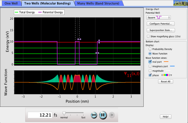
Figure 8.2:Bound states of a one-dimensional potential, with the well shape, depth, and width adjustable and the eigenfunctions drawn at their own energies. Superpositions of two eigenstates can be built and run in time, which is where the stationary states stop being stationary.
Interactive simulation: Quantum Bound States
Worked Example: Expectation Values in the Ground State
For the infinite-well ground state , the probability density is symmetric about the well’s midpoint , so by symmetry alone,
without needing to evaluate the defining integral explicitly — the particle is, on average, found at the center of the well, exactly as classical intuition would suggest, even though (unlike a classical particle) it is never actually found moving through the center with a definite velocity. By the same symmetry, : the stationary state carries no net probability current in either direction. However, : since the ground-state energy is purely kinetic ( inside the well), , so . The particle has a nonzero typical momentum magnitude, , even though its average momentum is zero — a direct, quantitative illustration of the uncertainty principle at work: a particle confined to width cannot have exactly, only with a nonzero spread , consistent with .
The Potential Step: Partial Reflection and Transmission
Before turning to bound states in a finite well, it is instructive to consider a simpler, unbound configuration: a potential step, for and for , with a particle of energy incident from . Classically, the particle simply slows down (its kinetic energy dropping from to ) as it crosses , but continues forward with certainty — transmission probability 1, reflection probability 0.
Quantum mechanically, the time-independent equation in each region gives oscillatory solutions, for (an incident wave of amplitude plus a reflected wave of amplitude ) and for (a transmitted wave only, since nothing is incident from ), with and . Matching and continuously at gives two equations in , , , which solve to
Because whenever (i.e., whenever ), some of the incident wave is reflected even though — a purely wave-mechanical effect (the same kind of partial reflection that occurs when light passes from one medium of different refractive index to another, Chapter 4) with no classical particle counterpart at all. Comparing probability flux (rather than amplitude) on the two sides gives the reflection and transmission coefficients,
the last equality expressing overall conservation of probability: every incident particle is eventually found either reflected or transmitted. If instead , then becomes imaginary, the “transmitted” solution turns into a decaying exponential (no propagating wave in region II at all), and exactly — total reflection, as classically expected — but, just as in the wave-packet argument of Chapter 7, the wave function does not vanish abruptly at ; writing with real, the wave function in region II becomes , decaying with a characteristic penetration depth rather than vanishing abruptly at . The particle therefore has a small but nonzero probability of being found some distance into the classically forbidden region, even though it is certain, eventually, to be reflected back the way it came — a preview of the tunneling phenomenon developed below, in which a second boundary, ending the forbidden region before has fully decayed away, allows the particle to escape entirely rather than merely penetrate and return.
Both halves of that story — partial reflection at a step the particle has the energy to cross, and exponential decay into a step it does not — can be run against a real wave packet rather than a plane wave in Figure 8.3. Send a packet at a step with and it visibly splits: part of it continues, slower and stretched, and part comes back, with the areas under the two pieces reproducing the and computed above. Lower the energy below and the packet is entirely reflected, but during the encounter it leaks a decaying tail into the barrier. Replacing the step by a barrier of finite thickness — the simulation’s next potential — is the whole of tunneling: the tail reaches the far side before it has died away, and what emerges there is a transmitted packet.
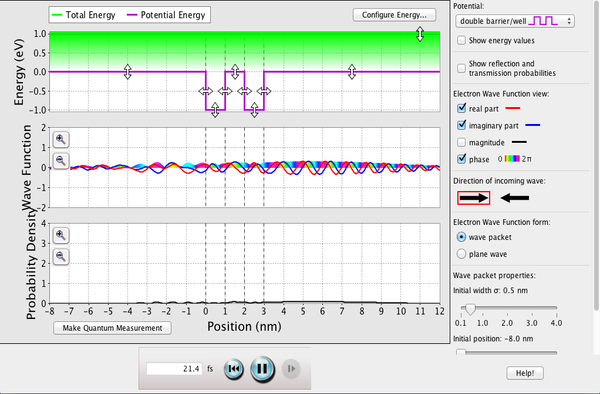
Figure 8.3:A wave packet incident on a step, a barrier, or a double barrier, with the real and imaginary parts of and the probability density all available. The energy relative to the barrier height is adjustable, as are the barrier’s width and height — the two parameters the transmission coefficient of the next section depends on exponentially.
Interactive simulation: Quantum Tunneling and Wave Packets
Worked Example: Reflection at a Potential Step
An electron with kinetic energy approaches a potential step of height . Since (with the same proportionality constant on both sides, as is unchanged), the ratio . The reflection coefficient is then
so about of an incident beam of such electrons is reflected by the step, and is transmitted — a small but entirely real and measurable effect, with no analog for a classical particle rolling over a downward step in a potential energy landscape.
8.3Tunneling, the Oscillator, and Correspondence
The Finite Square Well and Quantum Tunneling
A more physically realistic bound-state model replaces the infinitely high walls of the square well with walls of finite height : for and outside. For a bound state with , the time-independent equation outside the well becomes with real, whose normalizable solutions are decaying exponentials, moving away from the well, rather than the oscillatory sines and cosines found inside.
This is the central qualitative difference from the infinite well: the wave function does not vanish at the walls, but decays exponentially into the classically forbidden region where — a region a classical particle could never enter, since it would require negative kinetic energy there. Quantum mechanically, there is a small but nonzero probability of finding the particle just outside the well. Matching and continuously at each wall (rather than forcing as in the infinite well) yields a transcendental equation for the allowed energies, which must generally be solved numerically or graphically. Choosing the well symmetrically, for , exploits the potential’s reflection symmetry to separate the bound-state solutions into two families: even solutions, inside the well (), for which matching to the exterior decay gives the condition
and odd solutions, inside the well, for which the matching condition is instead
Because and are both functions of the single unknown , each of these is a single transcendental equation in , most easily solved graphically by plotting both sides as functions of and reading off the intersections; each intersection is one allowed bound-state energy. The lowest bound state is always of the even type (a symmetric, node-free wave function, exactly like the infinite well’s ground state); qualitatively, the finite well has fewer bound states than the infinite well of the same width, although a one-dimensional attractive finite well always has at least one bound state for any nonzero depth. Each allowed energy is slightly lower than the corresponding infinite-well value, because the wave function’s penetration into the forbidden region effectively widens the well.
This same exponential penetration underlies quantum tunneling: if a particle of energy encounters a finite-width barrier of height (rather than an infinite wall), the wave function decays but does not necessarily reach zero before the barrier ends, re-emerging on the far side as a (reduced-amplitude, but nonzero) oscillatory wave. There is then a nonzero probability — the transmission coefficient — that the particle is found on the far side of the barrier, despite lacking, classically, enough energy to pass over it. For a barrier of width and height , in the regime where the barrier strongly suppresses transmission (),
showing that tunneling probability falls off exponentially with both the barrier’s width and the square root of — which is why tunneling is significant for light particles (electrons) through thin barriers but utterly negligible for macroscopic objects. Tunneling is not a mathematical curiosity; it is the mechanism behind alpha decay (Chapter 13), the scanning tunneling microscope, and (approximately) the operation of tunnel diodes.
Worked Example: Distance Sensitivity of a Scanning Tunneling Microscope
A scanning tunneling microscope (STM) images a conducting surface by scanning a sharp metal tip a fraction of a nanometer above it and measuring the tunneling current of electrons crossing the vacuum gap — a gap that acts as a potential barrier of height roughly equal to the metal’s work function, here taken as . The decay constant is
Since , increasing the tip–surface gap by just (one angstrom) changes the transmission probability, and hence the measured tunneling current, by a factor of
roughly an order of magnitude per angstrom of vertical displacement — exactly the extreme sensitivity that allows an STM to resolve individual atoms on a surface by tracking tiny changes in tunneling current as the tip scans across atomic-scale height variations.
Worked Example: Order-of-Magnitude Estimate for Alpha Decay
Alpha decay (Chapter 13) is understood as an alpha particle () tunneling through the Coulomb barrier confining it inside a heavy nucleus. As a rough, illustrative model, approximate this barrier as rectangular, with the alpha particle’s energy falling below the barrier height and an effective barrier width (real barriers are Coulombic, not rectangular, and a proper treatment integrates over the barrier’s actual shape — the Gamow factor — but the rectangular approximation captures the essential physics). Then
so the tunneling probability per attempt is
This tiny number is not the final answer for a decay rate; it must be combined with an assault frequency, the rate at which the alpha particle, rattling back and forth inside the nucleus at a speed of order across a nuclear diameter of order , “attempts” to escape — roughly . The decay rate is then of order , corresponding to a half-life of order for this choice of illustrative barrier parameters. Real alpha emitters span half-lives from microseconds to billions of years, entirely because depends exponentially on and : changing the barrier parameters by a modest amount changes , and hence the half-life, by many orders of magnitude — exactly the empirical pattern captured by the Geiger–Nuttall relation revisited quantitatively in Chapter 13.
The Quantum Harmonic Oscillator
A particle in a potential (with here the spring constant, not a wave number) is the quantum analog of the classical simple harmonic oscillator, and it is important beyond this specific system because any smooth potential, expanded in a Taylor series about a point of stable equilibrium, is approximately parabolic near that minimum — the harmonic oscillator is the generic first approximation for small oscillations about equilibrium in essentially any bound system, including the vibrations of a diatomic molecule (Chapter 12).
Solving the time-independent Schrödinger equation with this potential (the details require either a power-series method or an elegant operator technique, developed in more advanced treatments) yields an evenly spaced energy spectrum,
with the classical angular frequency of the corresponding classical oscillator. Two features stand out. First, unlike the square well, the spacing between adjacent levels, , is the same for every — a distinctive signature of the parabolic potential. Second, the ground state () has energy , called the zero-point energy: even in its lowest possible energy state, a quantum oscillator retains irreducible energy and motion, again a manifestation of the uncertainty principle (a particle at rest, at the exact bottom of the well, would have , forbidden by ).
The ground-state wave function, , is a Gaussian, peaked (unlike the classical oscillator, which spends most of its time near the turning points, where it moves slowest) at the center — another qualitative divergence from classical intuition that only disappears, via the correspondence principle, for large , where the quantum probability distribution begins to average out to resemble the classical one.
Excited harmonic-oscillator wave functions follow the same node-counting pattern already seen for the infinite well: has exactly nodes (points, other than the boundaries at infinity, where the wave function crosses zero), so (the Gaussian ground state) has none, has one node at , has two nodes symmetric about the origin, and so on — a general feature of one-dimensional bound-state wave functions (also true of the infinite well, where has interior nodes in addition to the two required zeros at the walls themselves) that provides a quick, qualitative check on whether a proposed solution corresponds to the ground state, first excited state, or a higher state, without needing to solve the full equation.
Transitions between harmonic-oscillator levels by absorption or emission of a photon obey the selection rule : an oscillating dipole (the physical mechanism by which a vibrating charged system couples to the electromagnetic field) can only connect states whose quantum numbers differ by exactly one, so the emitted or absorbed photon energy is always , the same fixed spacing regardless of which pair of adjacent levels is involved — a fact used directly in Chapter 12 to interpret the vibrational spectra of diatomic molecules, where (to the extent the harmonic approximation holds) all vibrational transitions cluster near a single characteristic frequency rather than spreading across many distinct energies.
Worked Example: Zero-Point Motion, Macroscopic Versus Molecular
The characteristic spread of the ground-state Gaussian wave function is . For a macroscopic oscillator — a mass on a spring with , so — this gives
many orders of magnitude smaller than even a proton’s radius (): zero-point motion is utterly unobservable for a macroscopic object, consistent with everyday experience that a spring at rest simply looks at rest. By contrast, a carbon monoxide molecule vibrating with (a typical molecular vibrational frequency, corresponding to the reduced mass and bond stiffness of the C–O bond) has
a few percent of the bond’s equilibrium length () — small, but not at all negligible, and precisely why zero-point vibrational motion has measurable consequences (a nonzero zero-point vibrational energy that must be included in molecular bond-energy calculations) for real molecules even though the analogous effect is entirely unobservable for a spring on a lab bench.
The Correspondence Principle Across Three Systems
The three systems solved in this chapter — the infinite well, the finite well with tunneling, and the harmonic oscillator — share a common thread despite their different mathematical detail: each has a nonzero, quantized ground-state energy set by the uncertainty principle, the finite well and oscillator allow the particle to be found in regions forbidden to a classical particle of the same energy, and each converges toward classical predictions in an appropriate limit. For the infinite well, closely spaced levels at large (where but the fractional spacing ) approach a quasi-continuous classical energy spectrum; for the harmonic oscillator, the large- probability distribution develops peaks near the classical turning points, where a classical oscillator spends most of its time, rather than the single central peak seen for . This is Bohr’s correspondence principle: quantum predictions must merge smoothly into classical ones in the limit of large quantum numbers (equivalently, macroscopic action large compared to ), and it serves as a valuable consistency check on any quantum-mechanical solution.
The same principle explains why quantum effects are unobservable for everyday macroscopic objects even though, formally, every object obeys the Schrödinger equation. A macroscopic pendulum or block on a spring has an enormous effective quantum number (its total energy, measured in units of , is astronomically large for ordinary masses, spring constants, and amplitudes), placing it deep in the correspondence-principle regime where quantized energy levels are spaced far too closely, relative to the total energy, to be distinguished from a continuum, and where the wave-packet spreading of Chapter 7 is negligible on any observable timescale. The three exactly solvable systems of this chapter are pedagogically valuable precisely because they are simple enough to solve exactly while still exhibiting, at small , the full richness of specifically quantum behavior — behavior that becomes progressively harder to detect, though never strictly absent, as a system’s size, mass, or energy grows toward the macroscopic scale.
8.4Summary
The wave function evolves according to the time-dependent Schrödinger equation; gives the probability density for finding the particle, per the Born interpretation, and must be normalized, single-valued, finite, and continuous. Expectation values of position and momentum are computed by sandwiching the position operator () or momentum operator () between and and integrating; Ehrenfest’s theorem shows these expectation values obey Newton’s second law, recovering classical mechanics as the average behavior of a narrow wave packet.
For time-independent potentials, separable stationary-state solutions satisfy the time-independent Schrödinger equation; requiring to be normalizable in a confining potential generically forces to take only discrete, quantized values, while an unconfined particle has a continuous spectrum of scattering states.
The infinite square well gives , a nonzero ground-state energy, and wave functions with interior nodes — all with no classical counterpart.
A potential step produces partial reflection even when the particle’s energy exceeds the step height, with and — a purely wave-mechanical effect.
The finite square well allows the wave function to penetrate into the classically forbidden region outside the well; the same mechanism, applied to a finite-width barrier, produces quantum tunneling, with transmission probability falling off exponentially with barrier width and , the basis of the scanning tunneling microscope’s extreme distance sensitivity.
The quantum harmonic oscillator has evenly spaced levels , a selection rule for radiative transitions, and a nonzero zero-point energy ; it is the generic small-oscillation approximation to any smooth potential near a stable minimum.
Bohr’s correspondence principle — quantum predictions merge into classical ones at large quantum numbers — is a recurring consistency check across all three model systems.
8.5Problems
Solution to Exercise 8.1 #
For an electron in a well, when is in nanometers. Thus
Because , the emitted energy is .
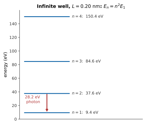
Figure 8.4:The spacing of infinite-well levels: the gap between and is , not , because .
Therefore, the ground-state energy is and the photon has energy .
Solution to Exercise 8.2 #
Solution to Exercise 8.3 #
The density is symmetric about , so its mean position is . The interior node follows from
for . Therefore, and the single interior node is at .
Solution to Exercise 8.4 #
For ,
For , , so and .
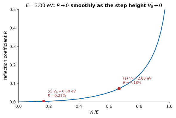
Figure 8.5: depends only on the ratio and falls smoothly to zero as ; both computed cases sit on this one curve.
Therefore, the reflection falls from to as the step is lowered.
Solution to Exercise 8.5 #
Solution to Exercise 8.6 #
Here . Using and ,
Thus . For an alpha particle, the mass is four times larger, so and .
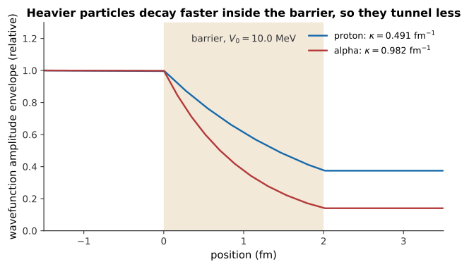
Figure 8.6:The heavier alpha particle has twice the proton’s decay constant , so its amplitude falls off twice as fast inside the barrier — the reason its transmission probability () ends up smaller.
Therefore, the proton transmission is about , while the alpha transmission is about because the heavier particle has a larger tunneling exponent.
Solution to Exercise 8.7 #
Tunneling current varies as , so an added gap changes it by
Therefore, a increase reduces the current by a factor of about 59, which is why STM height measurements can resolve much less than an angstrom.
Solution to Exercise 8.8 #
Solution to Exercise 8.9 #
The spacing is
Thus . An adjacent-level photon has and wavelength .
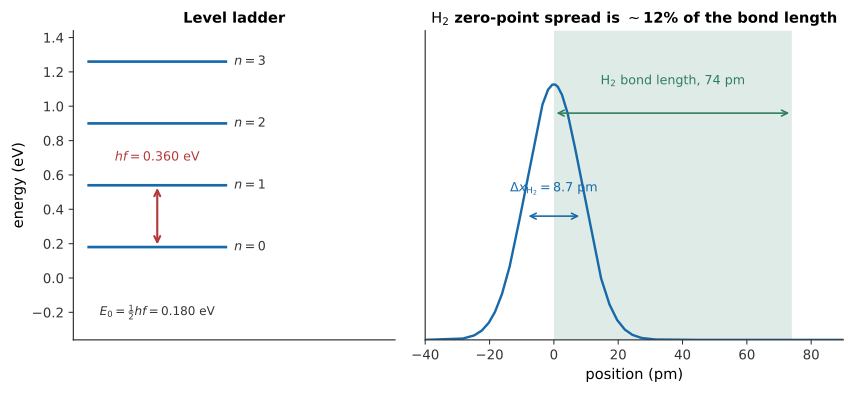
Figure 8.7:Left: the equally spaced ladder , with this problem’s zero-point energy and level spacing marked. Right: Problem 10’s zero-point position spread for H, , shown against the bond length it must fit inside.
Therefore, the zero-point energy is and vibrational transitions emit mid-infrared photons.
Solution to Exercise 8.10 #
For the oscillator, , so
For , and , shown to scale against the bond length in Figure 8.7. Therefore, the molecular zero-point spread is about of the bond length, whereas the macroscopic spread is negligible.
Solution to Exercise 8.11 #
Confinement requires a finite position uncertainty , which by requires nonzero momentum uncertainty and therefore positive kinetic energy. An oscillator likewise cannot have both exact equilibrium position and zero momentum. Therefore, both systems have a ground-state energy above the classical minimum; for macroscopic masses the resulting quantum energy is far too small to observe.
Solution to Exercise 8.12 #
The selection rule is . Starting at , the only downward one-photon transition is , and
The transition has and is forbidden for a single photon.
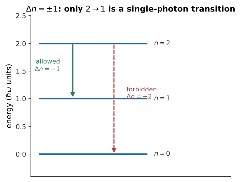
Figure 8.8:Only transitions emit or absorb a single photon; the direct path is forbidden regardless of how much energy it would release.
Therefore, the only allowed emitted photon has energy .
Solution to Exercise 8.13 #
A classical oscillator moves slowest near its turning points and fastest through , so it spends most of its time near the turning points. The correspondence principle requires the averaged probability density of a large- quantum state to reproduce that classical time distribution.
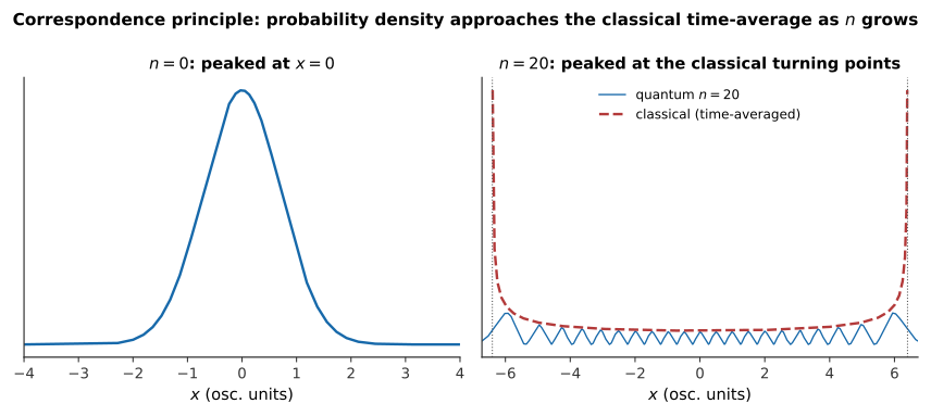
Figure 8.9: is peaked at the center, the opposite of the classical expectation. By , the fine quantum oscillations average out to the classical time-averaged density (dashed), which piles up at the turning points where the classical oscillator moves slowest.
Therefore, highly excited oscillator states have their largest probability density near turning points and their smallest near the origin.
Solution to Exercise 8.14 #
When , the wave number beyond the step is imaginary, so that region has no propagating wave capable of carrying transmitted probability current; hence . The acceptable solution there is nevertheless an exponentially decaying evanescent wave. Therefore, reflection is total even though the probability density penetrates a finite distance into .
Solution to Exercise 8.15 #
The probability density has three lobes and two interior nodes, at and ; the walls are additional zeros. Since ,
Therefore, the state has two interior nodes and its energy becomes one-quarter as large when the well width doubles.
Solution to Exercise 8.16 #
A plane wave has constant , so diverges and no finite normalization constant exists. It has one exact wave number and momentum , which requires completely indefinite position. Therefore, non-normalizability is the unavoidable position-space consequence of perfectly sharp momentum.
Solution to Exercise 8.17 #
At fixed width, increasing increases . In , a larger right-hand side allows intersections on additional tangent branches, each corresponding to another bound-state energy.
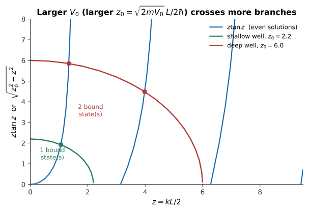
Figure 8.10:The matching condition plotted graphically: each branch of that the quarter-circle reaches gives one even bound state. Since , a deeper well (larger circle) reaches farther out and crosses more branches — here, one branch for the shallow well and two for the deep well, among the even-parity solutions alone.
Therefore, a deeper finite well supports more bound states.
Solution to Exercise 8.18 #
The worked example gives . For ,
With assault frequency , the decay rate is about and . Therefore, increasing the width by only changes the model half-life from about to about , illustrating the exponential sensitivity.
Solution to Exercise 8.19 #
The harmonic-oscillator state has exactly nodes, so has four. The infinite-well state has interior nodes, so its state also has four interior nodes. Thus, both specified states have four nodes in the stated convention: the infinite well’s two fixed wall zeros are not counted as interior nodes, and its positive-integer label is consequently one greater than the number of interior nodes.
Solution to Exercise 8.20 #
For large , , so
The spacing is negligible beside the pendulum energy. Therefore, the pendulum occupies a quantum number of order 1030 and its quantization appears completely continuous and classical.