Learning Objectives
By the end of this chapter, you should be able to:
Explain diffraction as the Huygens–Fresnel principle applied to a continuum of sources across a finite aperture, and say precisely how it differs — and does not differ — from the interference of Chapter 4.
Distinguish Fresnel (near-field) from Fraunhofer (far-field) diffraction, and decide which applies in a given geometry.
Derive the single-slit minimum condition by the pairwise-cancellation argument, and explain why is excluded.
Sketch and use the single-slit intensity pattern, including the width of the central maximum and the rapid decline of the secondary maxima.
Explain how a real double slit’s pattern is the product of a two-slit interference factor and a single-slit envelope, and locate missing orders.
Apply the grating equation, compute angular dispersion, and use the resolving power in spectroscopic problems.
Apply the Rayleigh criterion for a circular aperture to telescopes, microscopes, and the eye, and distinguish the diffraction limit from practical limits such as atmospheric seeing.
State Bragg’s law, use it to extract interplanar spacings from measured X-ray diffraction angles, and explain why the same argument applies to electron and neutron beams.
Describe how a hologram records and reconstructs a wavefront, and explain why it requires a coherent source.
Use single-slit diffraction to make a first, order-of-magnitude argument for the uncertainty principle of Chapter 7.
Introduction
In 1818 the French Academy of Sciences held a prize competition on the nature of light. Augustin-Jean Fresnel submitted a wave theory. Siméon Denis Poisson, a member of the judging committee and a convinced supporter of Newton’s particle theory, worked through Fresnel’s mathematics and triumphantly produced what he took to be its refutation: if Fresnel were right, then the shadow of a small circular disk, illuminated by a point source, would have a bright spot at its exact center — light would diffract around the rim, arrive at the axis having traveled equal distances from every point of that rim, and interfere constructively. The prediction was patently ridiculous.
A member of that committee, François Arago, went and looked. The spot was there.
That bright point — now called the Poisson spot, or the Arago spot, depending on whose role in the story one prefers to emphasize — is a fair emblem for this chapter. Diffraction is what waves do when they encounter an obstacle or a finite aperture: they bend into the geometric shadow, and they interfere with themselves in the process, producing patterns of light and dark that no ray-tracing argument can generate.
Chapter 4 worked with idealized slits: point-like Huygens sources, infinitesimally narrow, contributing one wavelet apiece. A real slit has a finite width , and every point across that width emits a wavelet. Summing those contributions is the whole subject of this chapter. Three results follow, in increasing order of consequence. First, a single slit, all by itself, produces a pattern of bright and dark bands. Second, real multiple-slit devices — above all the diffraction grating — combine the sharp interference maxima of Chapter 4 with a diffraction envelope that decides how bright each of those maxima actually is. Third, and most importantly, because every real optical instrument gathers light through an aperture of finite size, diffraction sets an absolute limit on the fineness of detail any instrument can resolve — a limit that no improvement in polishing, alignment, or manufacture can evade, because it is imposed by the wavelength of light itself.
5.1Diffraction Basics and the Single Slit
Diffraction Versus Interference: A Note on Words
It is worth settling a piece of vocabulary that causes more confusion than it should.
There is no physical distinction between interference and diffraction. Both are the same thing: coherent waves from different places arriving at a common point and adding as fields. The words differ only in bookkeeping convention. When the sources are a small, discrete set — two slits, five slits — the custom is to say interference and to write a sum. When the sources form a continuum across an aperture, the custom is to say diffraction and to write an integral. Richard Feynman put it bluntly: “no one has ever been able to define the difference between interference and diffraction satisfactorily. It is just a question of usage, and there is no specific, important physical difference between them.”
The reason the distinction survives is practical. In a real double slit there are two length scales — the slit separation and the slit width , with — and they produce structure on two very different angular scales. Calling the fine structure “interference” and the coarse envelope “diffraction” is a convenient way to keep track of which is which. That is all it is.
The Huygens–Fresnel Principle
Fresnel’s contribution was to make Huygens’s construction quantitative. Where Huygens drew an envelope of wavelets, Fresnel insisted on adding the wavelets as waves, with their phases, and then squaring the result to get an intensity. Stated for an aperture:
Every point of an open aperture acts as a source of secondary wavelets of equal amplitude and of the same phase as the incoming wave at that point. The field at any observation point is the sum, over the whole aperture, of these wavelets, each with the phase it has accumulated on its journey.
This Huygens–Fresnel principle reproduces the results of Chapter 4 when the aperture is a set of very narrow slits, and everything in this chapter when it is not. The sum becomes an integral, but the physics — add fields, account for phase, then square — is unchanged.
Near Field and Far Field
Whether the sum is easy or hard depends on the geometry, and the distinction matters enough to have names.
If the screen is far enough away that the rays converging on any observation point are effectively parallel, the phase of each wavelet is a linear function of its position in the aperture, and the integral is elementary. This is Fraunhofer diffraction, or far-field diffraction, and it is the case treated throughout this chapter.
If the screen is close, the rays are noticeably non-parallel, the phase varies quadratically across the aperture, and the pattern depends in a complicated way on distance. This is Fresnel diffraction, or near-field diffraction. The Poisson spot of the introduction is a Fresnel phenomenon; so are the fine bright and dark bands you can see just inside the edge of a sharp shadow cast by a small bright source.
The dividing line is set by the Fresnel number
where is the aperture size and the aperture-to-screen distance. Fraunhofer diffraction applies when ; Fresnel diffraction when . For a slit, light, and a screen away, , comfortably in the far field. Conveniently, a lens converts the far field into something you can put on a bench: any lens placed after the aperture brings the parallel bundles to a focus in its focal plane, so the Fraunhofer pattern appears there no matter how short the bench.
Single-Slit Diffraction
Consider a slit of width illuminated by a plane wave of wavelength , with a distant screen. The clever step, due to Fresnel, is not to attempt the whole sum at once but to ask a narrower question: in which directions does everything cancel?
Divide the slit conceptually into two equal halves, each of width , as in Figure 5.1(a). Pair up the topmost point of the upper half with the topmost point of the lower half; they are a distance apart. Pair the second point of the upper half with the second point of the lower half; also apart. Every point in the upper half has a partner in the lower half exactly below it. If the light heading off at angle from each pair is exactly out of phase — path difference — then every pair cancels, and so does the whole slit:
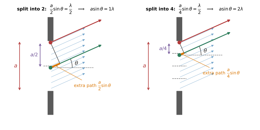
Figure 5.1:Canceling the slit against itself. Dividing the slit into two strips pairs each point with a partner away; when those pairs are a half wavelength out of step, the whole slit cancels, giving . Dividing into four strips pairs points apart and gives , and so on. Original schematic generated with matplotlib; see scripts/figures/.
Repeat the argument with four strips (Figure 5.1(b)): now partners are apart, each pair cancels when , and the whole slit cancels at . With strips the condition is . The complete set of single-slit minima is therefore
Two things about this formula regularly trip people up, and both are worth stating explicitly.
It locates minima, not maxima. Compare with the double-slit condition , which locates maxima. The two formulas look almost identical and mean opposite things. The distinction is not a convention: it comes from the fact that the pairing argument can only ever demonstrate cancellation.
is excluded. At every point of the slit is in phase with every other, so the wavelets add rather than cancel — there is nothing to pair against. The center of the pattern is a broad, bright central maximum, not a minimum. Formally, the pairing argument demands a path difference of within each pair, and supplies a path difference of zero.
The Width of the Central Maximum
The central maximum is bounded by the first minima on either side, at . Its angular half-width is therefore
exactly the scaling that the dimensional argument of Chapter 4 demanded. Note that in the central maximum runs from to , while every other maximum spans only : the central peak is twice as wide as the rest, in addition to being far brighter.
The most important qualitative consequence is that narrowing the slit widens the pattern, as Figure 5.2 shows.
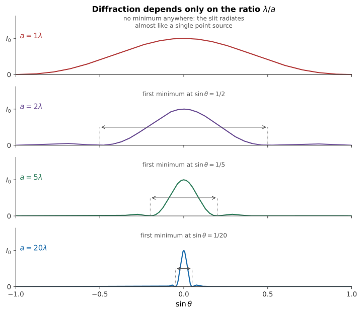
Figure 5.2:Single-slit patterns for four slit widths. The central maximum spans , so it narrows as the slit widens: a slit across concentrates the light into a beam, while a slit only across has no minimum at all and radiates almost like a single point source. Generated with matplotlib; see scripts/figures/.
This is the opposite of the naive expectation that a narrower opening should produce a narrower beam, and it is a genuinely wave-like signature. It also gives the correct picture of the limiting case: when , the condition has no solution, there are no minima anywhere, and the slit radiates into the entire forward hemisphere — behaving, exactly as Chapter 4 assumed, like a single Huygens point source. That is the justification, after the fact, for treating the slits of the double-slit experiment as points.
The inverse relationship between the aperture and its pattern is worth seeing rather than reading about, and Figure 5.3 shows the two side by side: the aperture on the left, the far-field pattern it produces on the right, with the aperture’s size and the wavelength both on sliders. Shrinking the opening spreads the pattern, and by exactly the ratio derived above. Two further controls make the point sharper than a single slit can. Squashing the round aperture into an ellipse produces an elliptical pattern elongated along the other axis, so the reciprocity holds direction by direction and not just on average; and the non-circular shapes on offer produce patterns of matching symmetry — an anticipation of the circular-aperture section below, where a round hole is found to give rings rather than a row of bands, and of the crystal lattices at the end of the chapter, where a periodic array of holes gives a periodic array of spots.
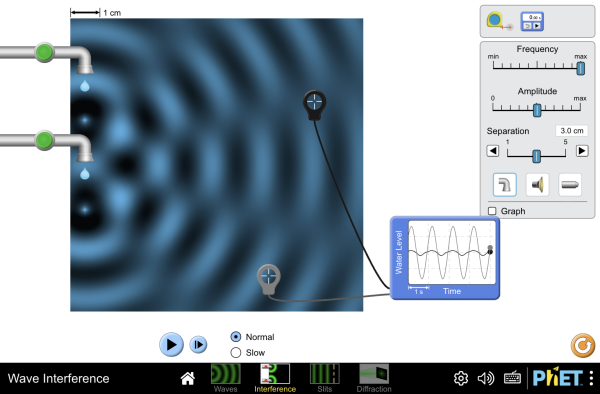
Figure 5.3:An aperture and the far-field diffraction pattern it produces, with aperture size, shape, and wavelength adjustable. Everything narrow in the aperture is wide in the pattern, and vice versa — the scaling of this section, seen whole rather than one angle at a time.
Interactive simulation: Wave Interference
Worked Example: Width of the Central Maximum
A slit of width is illuminated with light, and the pattern is observed on a screen away. Find the width of the central maximum.
The first minima are at
so (the small-angle approximation is excellent here). On the screen,
and the central maximum, running from to , has full width
Check the trend: halving the slit width to would double this to .
Worked Example: A Slit Too Narrow to Have Minima
At what slit width does the first minimum disappear entirely, for ?
The first minimum requires , so it exists only if . A slit narrower than one wavelength produces a smooth, minimum-free spread of light across the whole forward direction. Slits this narrow are difficult to make and transmit very little light, which is why the textbook idealization of a “point source slit” is easier to draw than to build — and why real double-slit experiments always show the envelope discussed below.
5.2Intensity Patterns and the Double Slit
Intensity in Single-Slit Diffraction
The pairing argument gives the zeros; getting the full curve requires actually doing the sum. The phasor picture of Chapter 4 makes this almost graphical.
Divide the slit into narrow strips and let . Each strip contributes a tiny phasor of the same length, and each is rotated slightly relative to its neighbor, because it sits slightly farther along the slit and so contributes a slightly different path. Let be the total phase difference between the wavelet from one edge of the slit and the wavelet from the other:
The chain of tiny phasors therefore turns through a total angle from beginning to end. A chain of equal segments turning at a uniform rate is an arc of a circle, and the resultant field is its chord (Figure 5.4).
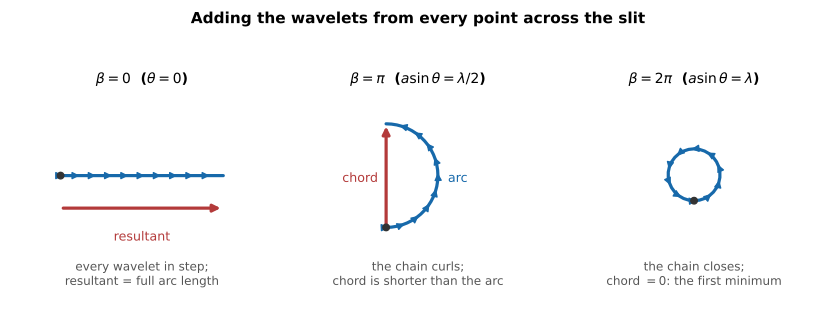
Figure 5.4:The single-slit phasor construction. The wavelets from across the slit form a chain of equal phasors turning through a total angle . At the chain is straight and the resultant equals the full arc length. As grows the chain curls and the chord falls behind the arc. At the chain closes into a circle and the resultant vanishes — the first minimum, . Original schematic generated with matplotlib; see scripts/figures/.
Everything follows from the geometry of a circular arc. Let the arc length be (this is the resultant at , when the chain is straight). An arc of length subtending angle has radius , and the chord across it is . So
and squaring gives the single-slit intensity pattern
The quantity in brackets is , where , so the pattern is often written .
Three checks confirm this is the right answer:
At , and , giving : the central maximum.
whenever with a nonzero integer, i.e. — precisely the pairing-argument minima. The case is excluded automatically, because rather than 0 there.
The chord can never exceed the arc, so everywhere.
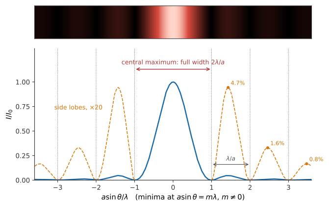
Figure 5.5:Single-slit diffraction intensity. The central maximum is twice as wide as the side lobes and vastly brighter — the first side lobe reaches only of the peak, so it is shown here magnified . The strip above shows the pattern as it appears on a screen, with faint bands brightened so they reproduce. Generated with matplotlib; see scripts/figures/.
The Secondary Maxima
Where are the maxima between the zeros? Setting gives the transcendental condition , which has no closed-form solution. Solving numerically puts the secondary maxima at
slightly inside the naive halfway positions , , — pulled toward the center because the envelope is falling. Relative to the central peak, the first three secondary maxima reach only
of , falling off roughly as . This is why a single-slit pattern does not look like a row of comparable fringes at all: it looks like one dominant bright band, flanked by faint ripples that most observers overlook entirely. It is also why Figure 5.5 has to magnify them before they are visible on the page.
Double-Slit Diffraction: Both Effects Together
Now put the two chapters together. A real double slit consists of two openings, each of finite width , whose centers are separated by . Both effects operate at once, and — because the field from each slit is the single-slit field, and the two slits then interfere — the intensities simply multiply:
Since , the factor oscillates rapidly and the factor varies slowly: fine fringes under a broad envelope, as in Figure 5.6.
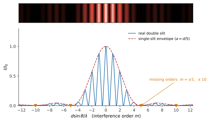
Figure 5.6:A real double slit with . The rapid fringes are set by the slit separation ; the dashed envelope is the single-slit pattern set by the slit width . Orders and vanish because they coincide with zeros of the envelope. Generated with matplotlib; see scripts/figures/.
Missing Orders
The striking feature of Figure 5.6 is that some interference maxima are simply absent. An interference maximum at is wiped out if a diffraction minimum, , falls at the same angle. Dividing one condition by the other, this happens when
that is, whenever is an integer. If is itself an integer, every -th order is missing — for the missing orders are , exactly as in the figure. If is a ratio of small integers, say , orders that are multiples of 5 still vanish but nothing else does. If is irrational, no order is exactly missing, though those near an envelope zero are suppressed almost to nothing.
Missing orders are a measurement, not a curiosity. Counting how many interference fringes fit inside the central diffraction maximum can reveal , without measuring either or : the central envelope spans and fringes are spaced by in . When is an integer, the visible orders are , giving bright fringes inside the central envelope; the orders at are missing at its edges. For a noninteger ratio, use the integer orders satisfying instead; the count then gives the corresponding integer bound, while the missing-order pattern can identify a rational ratio. Looking at a laboratory double-slit pattern and counting bright fringes between the first envelope zeros is therefore a genuine measurement of a ratio of two dimensions far too small to measure with a ruler.
Worked Example: Reading a Double-Slit Pattern
A double slit has slit width and separation , illuminated at . (a) Which orders are missing? (b) How many bright fringes lie inside the central diffraction maximum? (c) Find the angular width of the central envelope.
(a) , an integer, so orders are missing.
(b) The central envelope runs from to ; the fringes at its edges are the missing . The visible orders inside are : nine bright fringes, of which the central one is brightest.
(c) , so the envelope’s first zeros are at , giving a full angular width of . On a screen away that is a central band wide, containing nine fringes spaced apart — a comfortable laboratory pattern.
5.3Diffraction Gratings
A diffraction grating is the -slit device of Chapter 4 built for real: thousands of parallel slits per millimeter, ruled onto glass (a transmission grating) or onto a reflective surface (a reflection grating, which is what most modern spectrometers use). A compact disc is an accidental reflection grating, its data tracks spaced apart; a DVD’s tracks are apart, which is why it throws colors more widely.
Everything derived for ideal slits carries over. The principal maxima satisfy the grating equation
with the spacing between adjacent rulings; their width scales as and their peak intensity as . What is new is only that is now enormous — a beam on a grating with 600 lines per millimeter illuminates 6000 lines at once — so the maxima are not fringes but needle-sharp spectral lines. And of course the finite width of each opening imposes a diffraction envelope, exactly as for the double slit, so some orders are weak or missing. (Precision gratings are blazed: each groove is cut at an angle chosen to steer the envelope’s peak into a chosen order, so that most of the light ends up where it is wanted rather than in the useless direction.)
Dispersion
Because the diffraction angle depends on , a grating spreads white light into a spectrum — one spectrum per order, on each side of the center. Differentiating the grating equation gives the angular dispersion
so the spectrum spreads out more in higher orders and with finer rulings. It also shows that the orders eventually overlap: the red end of order can fall on top of the blue end of order , which is why spectrometers often place a coarse filter in front of the detector to isolate a single order.
Since , the mathematical upper bound on the order is — a grating so fine that produces no spectrum at all beyond . If is exactly an integer, that limiting order is at grazing angle () and is not usable in an ordinary detector geometry.
Resolving Power
The property that makes gratings scientific instruments rather than ornaments is their resolving power: the ability to display two nearly equal wavelengths as two separate lines rather than one blur.
Adopt the Rayleigh criterion — two lines are just resolved when the principal maximum of one falls on the first zero of the other. The principal maximum for wavelength in order sits at , and its first zero is away in angle. The line at sits away. Setting these equal,
Figure 5.7 shows the criterion in action. The resolving power depends only on the order and on the number of lines actually illuminated. Two consequences are worth noting. First, resolving power improves with the illuminated width of the grating, not with the total number of lines ruled on it; underfilling a grating with a narrow beam throws resolution away. Second, working in second or third order doubles or triples the resolution, at the cost of dimmer lines and increased risk of overlapping orders — a trade every spectroscopist makes.
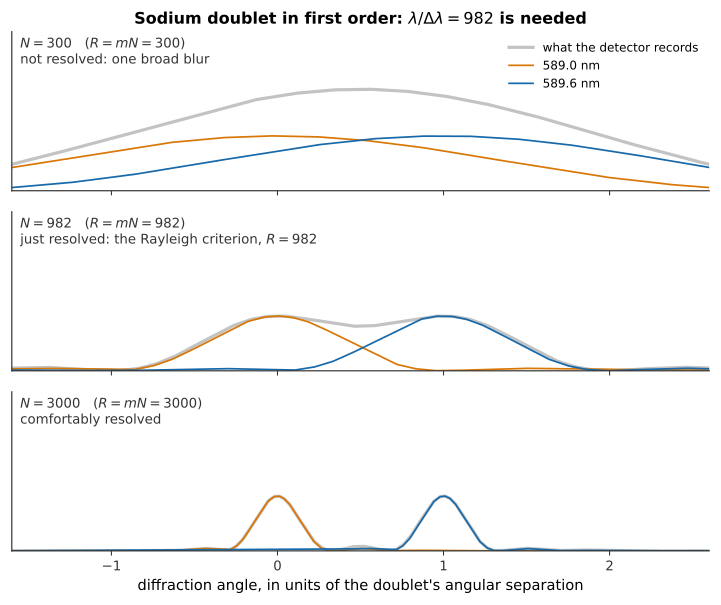
Figure 5.7:Resolving the sodium doublet (589.0 and 589.6 nm) in first order. With too few illuminated lines the two principal maxima are broader than their separation and merge into one feature. At , equals and the peak of one line falls on the first zero of the other — the Rayleigh criterion. With the lines are cleanly separated. Generated with matplotlib; see scripts/figures/.
Worked Example: Resolving the Sodium Doublet
The sodium doublet — the pair of yellow lines responsible for the color of a sodium street lamp — consists of lines at and . How many grating lines must be illuminated to resolve them in first order?
The required resolving power is
From with ,
On a grating with 600 lines per millimeter this needs a beam only wide — trivially met by any laboratory setup, which is why the sodium doublet is a standard first-week demonstration. In second order only 491 lines would be needed. By contrast, resolving the hyperfine structure within one of those lines requires a much larger resolving power than resolving the doublet — far beyond this simple demonstration and typically measured with specialized spectroscopic methods instead.
Worked Example: A Grating Spectrum
A transmission grating has 5000 lines per centimeter. (a) Find the line spacing. (b) Find the angle of the first-order maximum for . (c) Find the highest observable order. (d) Find the angular separation between the and hydrogen lines in first order.
(a) .
(b) , so .
(c) , but gives exactly — grazing emergence, unobservable in practice. The highest usable order is , at .
(d) and , a separation of . A grating spreads the visible spectrum over several degrees in first order — enough to project a spectrum across a wall.
5.4Resolution, Bragg Diffraction, and Holography
Circular Apertures and the Limits of Resolution
Every real optical instrument — a camera lens, a telescope mirror, a microscope objective, the pupil of the eye — collects light through a circular aperture of diameter . Its diffraction pattern is the circular analog of the single-slit pattern: a bright central disk, the Airy disk, surrounded by faint concentric rings.
The mathematics is harder than the slit case, because the integral runs over a disk rather than a line, and the answer involves a Bessel function rather than a sine. The structure of the result, however, is identical, differing only by a numerical factor that comes from the circular geometry: the first dark ring lies at
Compare this with for a slit. Nothing has changed except the 1.22 — which is, in fact, the first zero of the Bessel function divided by .
Where the factor 1.22 comes from
For a circular aperture of diameter , the far-field amplitude at angle is proportional to the two-dimensional analog of the single-slit integral, evaluated over a disk instead of a line:
where is the Bessel function of the first kind, order one — the circular-geometry replacement for the that came from integrating across a slit. This combination plays exactly the role played in the single-slit case: it equals 1 at zero argument, giving the central Airy peak, and has its first zero at the first zero of itself,
Substituting and and solving for ,
The extra factor, compared with a slit’s plain , is a purely geometric consequence of integrating over a disk rather than a line. No new physics enters — only a different shape of aperture.
The Rayleigh Criterion
Two distant point sources — two stars, or two features on a microscope slide — each produce their own Airy pattern in the image. If the sources are close together in angle, the two patterns overlap and merge into a single blob. Lord Rayleigh proposed a workable convention for where to draw the line: two sources are just resolved when the center of one Airy disk falls on the first dark ring of the other. That is, when their angular separation equals
Figure 5.8 shows what this looks like. At the criterion there is a shallow dip between the two peaks — about below the maxima. The criterion is a convention, not a law of nature: with a high signal-to-noise ratio and a known point-spread function, computational methods can do better, and some super-resolution fluorescence methods exploit temporal control or sparse emitters to distinguish features closer together than the Rayleigh separation. But as an estimate of what an instrument can do, it is excellent.
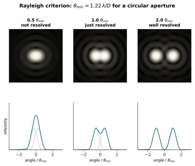
Figure 5.8:Two point sources imaged through a circular aperture, at separations of 0.5, 1.0, and 2.0 times , with intensity profiles beneath. At half the Rayleigh separation the pair is indistinguishable from a single elongated source; at the Rayleigh separation a shallow dip appears between the peaks; at twice it the two sources are unmistakable. Generated with matplotlib; see scripts/figures/.
The crucial thing about the Rayleigh criterion is its universality. It applies to every instrument with aperture , however perfectly made. It is not an engineering shortcoming to be designed away; it is a consequence of light having a wavelength and the instrument having an edge. The only levers available are and : use a shorter wavelength, or build a bigger aperture.
Both levers are pulled hard in practice. Telescopes get larger, and radio astronomers link dishes thousands of kilometers apart to synthesize an aperture the size of the Earth. Photolithography, which prints circuit features by projecting a mask onto a silicon wafer, has driven its light source from visible wavelengths down through deep ultraviolet to today’s extreme-ultraviolet at for exactly this reason. And electron microscopy takes the argument to its conclusion by abandoning light altogether in favor of electron matter waves whose wavelength (Chapter 7) can be a hundred thousand times shorter than visible light.
Worked Example: The Hubble Space Telescope
The Hubble Space Telescope has a primary mirror of diameter . (a) Estimate its diffraction-limited resolution at . (b) What is the smallest feature it could resolve on the Moon, away?
(a)
(b)
Hubble could not photograph the Apollo landing sites; the largest hardware left there is a few meters across. The limitation is not the telescope’s quality but its aperture, and no amount of image processing changes the fact that the information never entered the instrument.
Worked Example: The Eye, and Why Ground Telescopes Are Different
(a) The pupil of the eye is about in ordinary lighting. Its diffraction limit at is
At a reading distance of this corresponds to — about half the width of a human hair, and in reasonable agreement with measured visual acuity of about 1 arcmin. The eye is, remarkably, working close to its diffraction limit.
(b) Now apply the same formula to a telescope on the ground: arcsec, the same as Hubble. Yet ground-based images at visible wavelengths are typically blurred to about 1 arcsec, a factor of 17 worse. The culprit is not diffraction but atmospheric seeing: turbulent cells of air, of order across, refract the incoming wavefront by slightly different amounts and scramble it. The effective aperture is set by the turbulence, not the mirror. Two responses are possible — put the telescope above the atmosphere, which is why Hubble exists, or measure the distortion hundreds of times a second and cancel it with a deformable mirror, which is adaptive optics, and which now lets large ground telescopes reach their diffraction limits in the infrared.
This example is worth keeping in mind whenever a diffraction limit is quoted: it is a ceiling on performance, not a promise of it.
X-Ray Diffraction and Bragg’s Law
Gratings work because their line spacing is comparable to the wavelength of the light. To probe the arrangement of atoms in a solid, spaced a few tenths of a nanometer apart, we would need a grating with that spacing — and nature supplies one, in the form of a crystal, provided we bring a wave with a matching wavelength. That means X-rays, with .
Max von Laue proposed the experiment in 1912 and his collaborators Friedrich and Knipping performed it, obtaining a pattern of discrete spots from a copper sulfate crystal that established two things at once: that X-rays are waves, and that crystals are periodic arrays of atoms. Both had been conjectures until that afternoon.
W. H. Bragg and his son W. L. Bragg supplied the simple picture that made the technique usable, shown in Figure 5.9. Regard the crystal as a stack of parallel atomic planes separated by , and consider X-rays reflecting specularly from successive planes. By long-standing crystallographic convention, the angle is measured from the plane itself, not from the normal — a trap for anyone importing habits from optics.
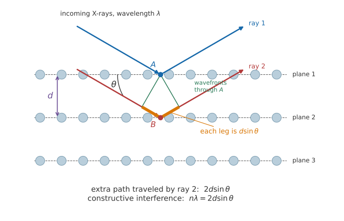
Figure 5.9:Bragg reflection. Two parallel X-rays strike successive atomic planes separated by . Relative to the wavefronts through , the ray reflecting from the lower plane travels two extra legs, each of length . Constructive interference requires the total, , to be a whole number of wavelengths. Original schematic generated with matplotlib; see scripts/figures/.
Ray 2 penetrates one layer deeper. Measured between the wavefronts through the point where ray 1 reflects, it travels two extra legs — one on the way in, one on the way out — each of length . Constructive interference between rays reflected from successive planes therefore requires
The consequence is that a crystal reflects a given X-ray wavelength strongly only at particular angles. Rotate a crystal in a monochromatic X-ray beam and the detector sees nothing at all until an angle satisfying Bragg’s law comes up, at which point a sharp peak appears. Measuring the set of such angles, for a set of crystal orientations, determines the spacings and symmetry of the atomic planes.
This is X-ray crystallography, and its record is hard to overstate: the structures of table salt and diamond (the Braggs, 1913), of penicillin and vitamin B (Dorothy Hodgkin), of DNA — the double helix inferred by Watson and Crick from the diffraction photographs taken by Rosalind Franklin and Raymond Gosling — and of hundreds of thousands of proteins since. Nearly everything we know about where atoms sit in condensed matter came through Bragg’s law.
The lattice on the other side of Bragg’s law is the subject of Figure 5.10. Changing the unit cell changes the set of atomic planes, their spacings , and therefore the angles at which reflections appear — including the aperiodic case, where the diffraction pattern is as sharp as a crystal’s but carries a symmetry no crystal can have.
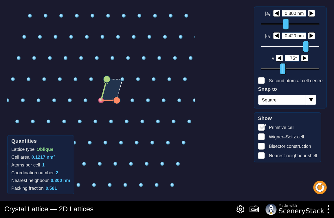
Figure 5.10:Crystal structure in five screens: the two-dimensional Bravais lattices, cubic unit cells, close packing, Miller indices, and aperiodic order. The Miller-index screen is the direct companion to Bragg’s law — it is where the planes of spacing come from.
Interactive simulation: Crystal Lattice
Worked Example: An Interplanar Spacing
X-rays of wavelength (the copper line, the workhorse of laboratory diffractometers) produce a first-order Bragg reflection at . Find the spacing of the reflecting planes, and find where the second-order reflection appears.
First order, :
a typical interatomic spacing. For ,
Note that a third order would require : with this wavelength and this spacing, only two orders exist. Requiring also shows why X-rays are essential — with visible light, and no order exists at all, which is exactly why crystals look like ordinary transparent solids rather than gratings.
Not Just X-Rays
Bragg’s law contains no reference to what kind of wave is diffracting. Any wave whose wavelength is comparable to the interplanar spacing will do — and by the time you reach Chapter 7, you will know that electrons and neutrons are such waves.
That is not a rhetorical flourish; it is the historical route by which matter waves were confirmed. In 1927 Clinton Davisson and Lester Germer fired low-energy electrons at a nickel crystal and found the scattered intensity peaking at exactly the angles Bragg’s law predicts, for a wavelength matching de Broglie’s . Neutron diffraction, which is sensitive to light atoms in a way X-rays are not, is now the standard way to locate hydrogen in a crystal structure and to map magnetic ordering. The same equation, first written for X-rays, ended up as one of the sharpest pieces of evidence for the wave nature of matter.
Holography
An ordinary photograph records intensity and throws away phase, which is why it is flat: all the information about the shape of the wavefront arriving from the scene is lost. A hologram, invented by Dennis Gabor in 1947, records the phase as well — by the only means available, namely by converting phase differences into intensity differences through interference.
The recording step splits a laser beam in two. One part, the object beam, illuminates the subject and scatters from it onto the film. The other, the reference beam, goes straight to the film. Where the two arrive in phase the film is exposed; where they arrive out of phase it is not. What the film records is therefore a dense, fine interference pattern — nothing resembling a picture, just an apparently random speckle of microscopic fringes — which encodes both the amplitude and the phase of the light arriving from every point of the object.
The reconstruction step is pure diffraction. Illuminate the developed film with the reference beam alone, and the recorded fringe pattern acts as a complicated diffraction grating, diffracting the reference beam into exactly the wavefront that the object originally sent out. An observer looking into the film sees that wavefront and cannot tell it from the object: it has full parallax, and looking around the edge of a foreground object reveals what is behind it.
Two properties follow directly from this account. First, holography demands a source with a coherence length longer than the depth of the scene, which is why it was impossible before the laser and why Gabor’s original demonstrations were so limited. Second, every part of the hologram receives light from every part of the object, so a hologram cut in half still reconstructs the whole scene — from a smaller effective aperture, and therefore, by the Rayleigh criterion, with correspondingly poorer resolution.
Looking Ahead: Diffraction and the Uncertainty Principle
There is one more thing to extract from single-slit diffraction, and it is the reason this chapter belongs in a book on modern physics.
Take the pattern seriously as a statement about photons. A photon that passes through a slit of width has, at that moment, a position along the slit known to within
It arrives traveling straight ahead, with no transverse momentum. Yet it lands somewhere within the central diffraction maximum, which means that on emerging it has acquired a transverse momentum of order , where is the angle to the first minimum. Using and the photon momentum (established in Chapter 6),
Multiply:
The width of the slit has canceled out. Squeeze the slit to pin down the photon’s position and the diffraction pattern widens by exactly enough to keep the product fixed; open it up and the reverse happens. There is no way to make both small at once — not because the measuring apparatus is clumsy, but because the light is a wave, and this relation is a property of waves.
This is the Heisenberg uncertainty principle, arrived at from nothing but classical wave optics and one quantum fact (). Chapter 7 derives it properly, shows that it applies to electrons and every other particle, and works out its consequences. But it is worth seeing now, in this chapter, that its origin lies in the ordinary mathematics of diffraction — that the strangest feature of quantum mechanics is, at bottom, the same phenomenon that spreads light behind a narrow slit.
5.5Summary
Diffraction and interference are the same physics — coherent waves added as fields. The words distinguish a continuum of sources (an integral) from a discrete set (a sum), and nothing more.
The Huygens–Fresnel principle treats each point of an aperture as a source of wavelets that are summed with their phases. Fraunhofer (far-field) diffraction applies when the Fresnel number , or whenever a lens is used to bring parallel bundles to a focus; Fresnel (near-field) diffraction applies otherwise, and produces effects such as the Poisson spot.
Single-slit minima occur at for nonzero integer , derived by pairing points apart so that every pair cancels. is excluded: the center is a broad maximum.
The single-slit intensity is with , obtained from the chord of the circular phasor arc. The central maximum has half-width , is twice as wide as the side lobes, and dominates: the first side lobe reaches only of the peak.
Narrower slits spread light more. For no minimum exists and the slit radiates like a point source, justifying the idealization of Chapter 4.
A real double slit gives the product : fine interference fringes set by , under a broad envelope set by . Orders for which is an integer are missing; counting the fringes inside the central envelope measures .
A diffraction grating obeys with angular dispersion and resolving power , where is the number of illuminated lines. Only orders up to exist.
A circular aperture of diameter produces an Airy pattern with first zero at . The Rayleigh criterion adopts this as the resolution limit of any instrument with that aperture — a fundamental diffraction limit, though real performance may be worse (atmospheric seeing) or, with enough signal and cleverness, better.
Bragg’s law, with measured from the atomic planes, governs constructive reflection from a crystal lattice. It underlies X-ray crystallography, and applies equally to electron and neutron waves — as Davisson and Germer showed in 1927 (Chapter 7).
A hologram records the interference between an object beam and a reference beam, capturing phase as well as amplitude; illuminating it with the reference beam diffracts a reconstruction of the original wavefront.
Applying and to a single slit gives : the uncertainty principle, already visible in classical diffraction.
5.6Conceptual Questions
State, in one sentence each, the physical difference between the conditions for a double slit and for a single slit. Why do two nearly identical formulas describe opposite things?
Explain, using the pairing argument, why can never be a diffraction minimum, no matter how many strips the slit is divided into.
A single slit is illuminated with red light, then with blue light. Which pattern is wider, and why? Now the same slit is made narrower. Which way does the pattern change? Are the two answers consistent with a single rule?
Explain why a wider telescope aperture improves angular resolution, while a wider slit narrows the diffraction pattern. These sound like opposite statements about what a bigger aperture does. Show that they are the same statement.
In a real double-slit pattern, some interference maxima are missing entirely. Explain what has happened to the light that “should” have been there, and why energy is nonetheless conserved.
Why can visible light not be used to determine crystal structures by Bragg diffraction? Answer quantitatively, using the constraint .
A hologram is cut in half. Explain why each half still reconstructs the entire scene, and what is degraded.
A camera lens is stopped down from to , reducing the aperture diameter by a factor of 8. Aberrations improve when a lens is stopped down, but diffraction gets worse. Explain the trade-off, and state which effect dominates at very small apertures.
5.7Problems
Solution to Exercise 5.1 #
Solution to Exercise 5.2 #
Solution to Exercise 5.3 #
At ,
The true first secondary maximum is , so the midpoint estimate is lower by , or about of the secondary-maximum value. Therefore, the halfway-point intensity is of the central maximum and is already a good approximation to the true secondary maximum.
Solution to Exercise 5.4 #
The Fresnel number is . Setting gives
Therefore, distances only of order are still at the Fresnel--Fraunhofer boundary; the far-field formulas require a screen appreciably farther away than this scale.
Solution to Exercise 5.5 #
The ratio is
An interference maximum is missing when , or . Up to , the missing orders are and . The central envelope contains , namely , for nine nonmissing bright fringes — exactly the pattern plotted in Figure 5.6, whose missing orders are this problem’s . Therefore, , orders 5 and 10 are absent, and nine bright fringes lie inside the central diffraction maximum.
Solution to Exercise 5.6 #
If is an integer , the central maximum contains the orders , a total of bright fringes. Hence
Therefore, the slit-separation-to-width ratio is .
Solution to Exercise 5.7 #
The line density is , so
For first order, , so . The largest order is . Differentiating gives
Therefore, the spacing is , the first-order angle is , the mathematical upper-bound order is 4, and the first-order dispersion is . The fourth order is at grazing angle, so the highest usable order is 3.
Solution to Exercise 5.8 #
Resolving power is . In second order,
In first order it is , twice as large, so the resolution is two times poorer. If only 1000 lines are illuminated in second order, and ; only illuminated lines contribute coherently, exactly as Figure 5.7 shows for the sodium doublet: raising narrows each order’s peak until two close wavelengths separate. Therefore, second order resolves versus in first order, and narrowing the beam reduces the resolving power in direct proportion to the illuminated line count.
Solution to Exercise 5.9 #
The spacing is . In first order the endpoint angles are and , so the width is . In second order they are and , so the width is .
Overlap begins where . The first common direction occurs for and , at or . The overlap ends where the second-order red limit is reached, at and (which corresponds to in third order).
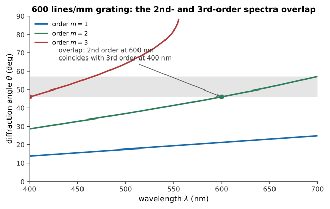
Figure 5.11:The three orders’ angular ranges as sweeps across the visible spectrum. The shaded band is where 2nd- and 3rd-order light arrive at the same angle; it begins where the 2nd order’s meets the 3rd order’s , both at .
Therefore, the first- and second-order widths are and , and second and third orders overlap from to .
Solution to Exercise 5.10 #
The Rayleigh limit is
At , . This is the “just resolved” case of Figure 5.8, where the two Airy patterns are separated by exactly . Therefore, the ideal eye resolves about , corresponding to at reading distance.
Solution to Exercise 5.11 #
Using ,
Therefore, diffraction alone would permit resolution to roughly . In ordinary viewing, the eye’s aberrations and retinal sampling usually make the practical limit less favorable; atmospheric turbulence can add further blur over long paths.
Solution to Exercise 5.12 #
Since , doubling changes the limit to . Halving from to at fixed also changes it to . Therefore, either modification improves the angular resolution by a factor of two.
Solution to Exercise 5.13 #
The half-angle subtended by the objective is , so in air its numerical aperture is (the small-angle estimate is close). Thus
At the same aperture angle, replacing by gives , an improvement by . Therefore, the light microscope resolves about and the electron microscope about under the stated idealized comparison.
Solution to Exercise 5.14 #
Bragg’s law is . For first order,
For second order, , so . Finally , so .
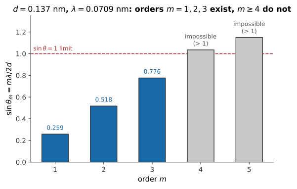
Figure 5.12: grows in equal steps with ; it crosses the physical ceiling between and , so no reflection of any order beyond exists for these planes.
Therefore, the plane spacing is , the second-order reflection is at , and orders through exist.
Solution to Exercise 5.15 #
For first order,
This is , in the X-ray region. Since , the longest diffracting wavelength is . Therefore, the required wavelength is and no wavelength longer than can produce a Bragg reflection from these planes.
Solution to Exercise 5.16 #
Bragg’s law requires . Because and the smallest order is , an order can exist only if . For , , whereas visible light has . Therefore, visible light is about 900 times too long in wavelength to diffract from atomic crystal planes.
Solution to Exercise 5.17 #
The first minimum of a narrow slit obeys , so decreasing makes the diffracted beam wider: localization at a smaller opening creates a larger angular spread. A telescope, however, uses a large aperture to make the diffraction pattern of each point source narrower, allowing two nearby patterns to be distinguished. Therefore, the statements are complementary rather than contradictory: a narrow aperture spreads one beam widely, while a large collecting aperture reduces the diffraction blur of an image.
Solution to Exercise 5.18 #
For , , hence . Taking and ,
so . For , the first minimum is at , , and the product is again . Therefore, halving the slit doubles the momentum uncertainty while leaving of order .
Solution to Exercise 5.19 #
The synthesized aperture has
Since , the shadow is just resolvable.
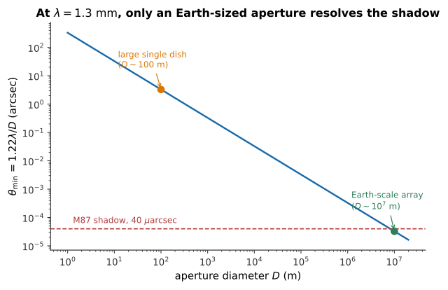
Figure 5.13:Angular resolution improves only as , so reaching at requires an aperture the size of the Earth; even the largest single dish () falls short by a factor of 105.
Therefore, Earth-scale interferometry provides just enough resolution, whereas a single dish would need an impossible diameter comparable to Earth to supply the same aperture.
Solution to Exercise 5.20 #
For a CD, and , so . The maximum order is . For a DVD, , so and .
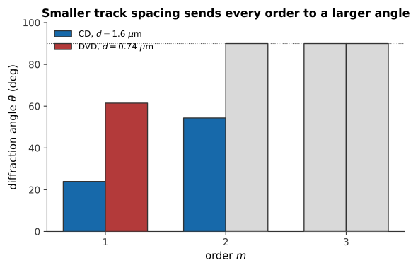
Figure 5.14:At the same wavelength, the DVD’s smaller track spacing pushes every order to a larger angle; its first order alone exceeds the CD’s, and no second order exists for the DVD at all, since there.
Therefore, a DVD sends the first order to a much larger angle than a CD, producing a wider color spread because its track spacing is smaller.