Learning Objectives¶
By the end of this chapter, you should be able to:
Substitute the Coulomb potential into the general radial equation of Chapter 9 to obtain the resulting energy quantization for hydrogen, and compare it to the Bohr model’s prediction.
Explain, from the normalizability of the radial equation’s solutions, why the principal quantum number is discrete and why is restricted to .
Write down the explicit hydrogen radial wave functions , , , describe the resulting radial probability distributions, and use the effective (centrifugal) potential to explain why low- states penetrate closer to the nucleus.
Extend the hydrogen solution to hydrogenic ions (e.g., , ) and compute the scaling of energy and scaling of orbital size.
Read an energy-level diagram for hydrogen and compute the wavelengths of lines in the Lyman, Balmer, and Paschen series.
Enumerate the allowed quantum states for a given and explain the origin of degeneracy in hydrogen.
Explain electron spin and the Stern–Gerlach experiment that revealed it, and compute the force and deflection produced by a Stern–Gerlach magnet.
Specify an electron’s orbital and spin orientation using the magnetic quantum numbers and , and compute the corresponding orbital and spin magnetic moments.
Compute the frequency and wavelength shift produced by the (normal) Zeeman effect, and estimate the order of magnitude of fine-structure splitting in terms of the fine-structure constant .
Apply selection rules to determine which transitions between hydrogen energy levels are allowed.
Introduction¶
Chapter 9 developed the general machinery for any central potential: separation into radial and angular parts, and the universal quantization of orbital angular momentum. This chapter specializes that machinery to the single most important central potential in atomic physics — the Coulomb attraction between an electron and a proton — and solves it for the hydrogen atom, the only atom for which the Schrödinger equation can be solved exactly in closed form. The result reproduces (and explains, rather than assumes) the energy levels first found empirically in atomic spectra and postulated ad hoc in the 1913 Bohr model, while revealing a far richer structure — angular momentum, spatial probability distributions, and a fourth quantum number, electron spin, with no classical counterpart at all.
10.1Energy Levels and Hydrogenic Structure¶
The Radial Equation and Energy Quantization¶
For the hydrogen atom, the central potential is the Coulomb attraction between the electron (charge ) and the proton (charge ),
Substituting this into the radial equation obtained from the separation (Chapter 9), and requiring to be normalizable (i.e., to decay rather than blow up as , and to remain finite at ), restricts the allowed energies to exactly the same discrete set found by Bohr in 1913 from an ad hoc semiclassical model:
This agreement is a triumph for the Schrödinger equation — it reproduces a result that matched atomic spectroscopy to remarkable precision — but the derivation and interpretation are entirely different from Bohr’s. Bohr postulated that the electron moves on definite circular orbits, with angular momentum quantized as by assumption. The Schrödinger treatment makes no such assumption about orbits at all; instead, emerges purely as an index counting the normalizable solutions of the radial equation, the electron has no well-defined trajectory, and — as shown below — the ground state () actually has zero orbital angular momentum, in direct contradiction to Bohr’s . The numerical agreement in is, in this sense, a coincidence specific to the particular form of the Coulomb potential, not a sign that the Bohr picture was substantially correct.
The mechanism behind the discreteness is worth making explicit, since the same pattern recurs throughout quantum mechanics. Solving the radial equation for a trial (negative) energy produces a function that falls off as at large , with , multiplied by an infinite series in powers of ; for almost any choice of , that series itself grows fast enough that the full product still diverges as , exactly the unnormalizable blow-up that ruled out most trial energies in the finite square well of Chapter 8. Demanding a normalizable wave function forces the series to terminate after a finite number of terms — collapsing it from an infinite series into a finite polynomial — and this termination happens only when lands exactly on a positive integer, which is precisely the principal quantum number . The same termination condition also caps the orbital quantum number: the polynomial’s degree fixes a nonnegative integer (the number of interior radial nodes, discussed further below) related to and by , so that immediately forces — and, for the ground state , forces exactly, which is the direct algebraic reason the ground state must have zero orbital angular momentum, not merely an empirical fact to be taken on faith.
The distance between Bohr’s picture and Schrödinger’s is easiest to see by running them side by side, as in Figure 10.1. Both reproduce the same and therefore the same emission lines, but only one of them places the electron on an orbit.
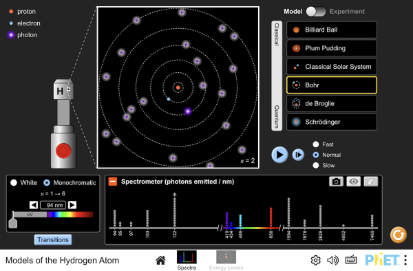
Figure 10.1:Successive models of the hydrogen atom — Bohr, de Broglie, Schrödinger, and their predecessors — each firing photons at an atom and producing a spectrum. The models that agree on disagree entirely about where the electron is.
Interactive simulation: Models of the Hydrogen Atom
Historical Context: Bohr’s 1913 Model and Its Limits¶
It is worth pausing on why a model built on postulates that turned out to be simply wrong — definite orbits, angular momentum quantized as — nonetheless earned Niels Bohr the 1922 Nobel Prize and remains the picture most people first encounter. In 1913, thirteen years before Schrödinger’s equation existed, Bohr combined classical circular-orbit mechanics with a single ad hoc quantization rule and reproduced the empirical Rydberg formula for hydrogen’s spectral lines essentially exactly, including its dependence on nuclear charge for hydrogenic ions (below) — a stunning success for a model with no derivation behind its central assumption. The de Broglie standing-wave argument of Chapter 7 later supplied a retroactive justification for , which is part of why the Bohr model survived as long as it did before being fully superseded.
The model’s failures, however, were just as instructive as its success. Extending Bohr’s orbit-quantization scheme to helium — even with the refinements (elliptical orbits, relativistic orbit precession) added by Arnold Sommerfeld through the 1910s — never produced a correct ionization energy or a stable ground-state configuration for a two-electron atom; the semiclassical machinery simply had no consistent way to handle two mutually interacting orbiting electrons. The model also could not predict which transitions between levels actually occur (the selection rules developed later in this chapter), could not account for the relative brightness of spectral lines, and — as already emphasized above — gets the ground state’s angular momentum flatly wrong: Bohr’s orbit carries , while the true ground state has and no orbit, well-defined trajectory, or definite radius at all, only the probability cloud shown in Figure 10.1. These failures, especially the inability to extend the model consistently beyond hydrogen, were a central motivation for the fully quantum-mechanical treatment developed in Chapters 8–9 and specialized to hydrogen in this chapter — a treatment that, unlike Bohr’s, generalizes cleanly to helium and every other atom in Chapter 11.
Hydrogenic Ions: Scaling with Nuclear Charge¶
Everything derived above specializes the general central-potential machinery of Chapter 9 to a nuclear charge of exactly . The same radial equation applies unchanged, with only in the Coulomb potential, to any hydrogenic (hydrogen-like) ion: a single electron bound to a nucleus of charge , such as singly ionized helium () or doubly ionized lithium (). Repeating the normalizability argument above with the rescaled potential gives
where is the characteristic Bohr length scale of the -th shell. It is useful for comparing orbital sizes, but it is not the exact radial-probability peak for every state; those peak positions also depend on . Both dependences make direct physical sense: a larger nuclear charge attracts the electron more strongly, pulling its orbit inward (radius shrinks as ) while binding it more tightly — and because the potential energy itself scales as while the resulting spatial compression compounds that scaling once more, the binding energy grows as , not simply . This scaling reappears with direct experimental consequence in Chapter 11, where it underlies Moseley’s law for the energies of characteristic X-ray transitions in multi-electron atoms.
Worked Example: The Ionization Energy and Orbital Size of He⁺¶
Find the ground-state ionization energy and the most probable electron–nucleus separation for (), a one-electron ion, and compare both to hydrogen’s.
so the ionization energy — the energy required to remove the electron entirely — is , exactly four times hydrogen’s , matching the measured ionization energy of . The orbital size scales the other way,
half of hydrogen’s Bohr radius: the electron in is bound four times more tightly and orbits, on average, twice as close to the nucleus as the electron in neutral hydrogen — both consequences of the same doubled nuclear charge, entering the energy quadratically and the size linearly (inversely).
Quantum Numbers and Degeneracy in Hydrogen¶
Solving the full three-dimensional problem gives states labeled by the same three quantum numbers introduced in Chapter 9 — , , — but with a further restriction, specific to the Coulomb potential, tying to :
Because the energy depends only on — not on or — every state sharing a given is degenerate (equal in energy), regardless of its orbital angular momentum. Counting the total number of combinations for a given gives degenerate states (before accounting for electron spin, discussed below): for example, admits (one state, ) and (three states, ), for states total. This -independence of the energy is itself notable — it does not hold for multi-electron atoms (Chapter 11), where the energy depends on as well as , and is a special feature of the pure Coulomb potential (technically, a signature of a hidden extra symmetry, beyond ordinary rotational symmetry, unique to the potential).
The Hidden Symmetry Behind ℓ-Independent Degeneracy
Ordinary three-dimensional rotational symmetry guarantees that energy cannot depend on , since no direction in space is special — but it says nothing about . A generic central potential’s energy levels do depend on , and indeed they do for every atom with more than one electron (Chapter 11). Hydrogen’s extra, “accidental” -independence traces back to a conserved quantity unique to the exact potential: the classical Laplace–Runge–Lenz vector,
which points from the focus of a classical Kepler orbit toward its perihelion and is constant in time only for a force that falls off as exactly — not , not . Quantum mechanically, becomes an operator that commutes with the Hamiltonian and connects states of different at the same , enlarging the symmetry governing hydrogen from ordinary three-dimensional rotations, , to a larger four-dimensional rotation group, , whose representations turn out to be exactly the -fold degenerate multiplets observed. This is the same underlying fact about the force law that makes classical Kepler orbits close on themselves without precessing — the classical and quantum “accidents” are one and the same.
10.2Wave Functions, Spectra, and Spin¶
Wave Functions and Probability Distributions¶
The full wave functions, , have structure worth examining qualitatively even without their explicit algebraic form. The ground state, , is spherically symmetric (, so is constant) and decays exponentially, , where
is the Bohr radius — reappearing here not as the radius of a Bohr orbit but as the natural length scale over which the ground-state probability density falls off. The radial probability distribution, (the probability per unit of finding the electron at distance from the nucleus, obtained by integrating over all angles at fixed ), peaks at for the ground state — the most probable electron-nucleus distance in hydrogen’s ground state is exactly the Bohr radius, even though the electron has zero orbital angular momentum and hence, unlike in the Bohr picture, is not “orbiting” in any classical sense.
Written out in full, with proper normalization, the lowest few radial wave functions are
each verified against the standard hydrogen wave-function table (e.g. OpenStax Vol. 3, §8.2). The pattern generalizes: every is an exponential (decay rate set only by ) multiplied by a polynomial in of degree , and the number of interior zeros of that polynomial — the radial nodes counted below — is exactly , the same integer introduced above via . () is a bare exponential with no node; () has one node, at , exactly where its parenthetical factor vanishes; (, since its higher “uses up” the node budget at fixed ) is a bare power of times an exponential, with no node at all despite sharing with .
Figure 10.2 plots the resulting for six low-lying states, making the node-counting rule directly visible rather than merely asserted: each panel’s dotted vertical lines mark its nodes, and the count in every panel matches exactly — zero for , , and ; one for and ; two for .
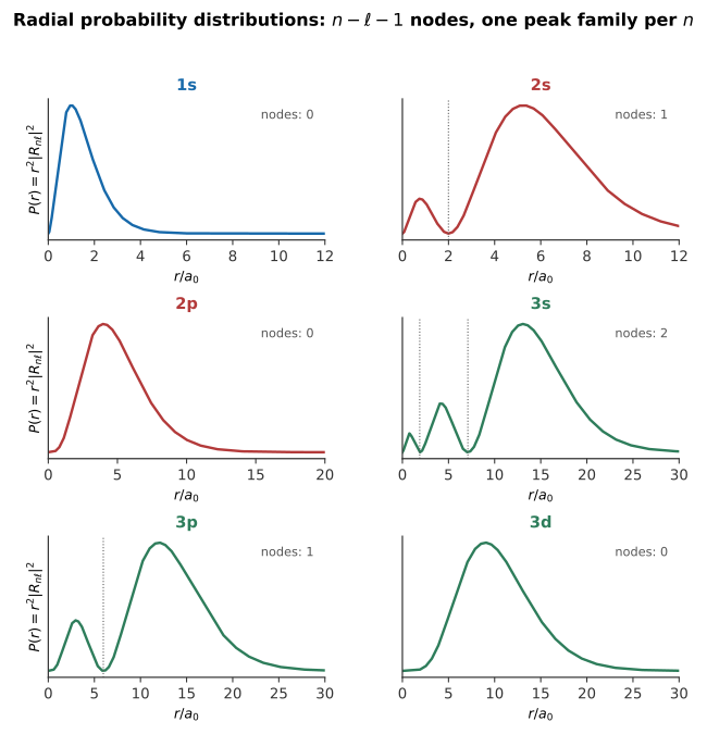
Figure 10.2:Radial probability distributions for the six lowest distinct combinations. Each state’s node count matches exactly, and every curve for a given extends, on average, farther from the origin as increases — the size of the atom really does grow with , just not along a sharp Bohr orbit. Computed directly from the closed-form formulas; see scripts/figures/.
More generally, has radial nodes (points, other than and , where the probability density vanishes), and the angular functions have angular nodes (nodal planes or cones) whose count and shape depend on and — giving rise to the familiar (spherical), (dumbbell-shaped, with a single nodal plane through the origin), and -orbital shapes used throughout chemistry (Chapter 12) to describe electron distributions in atoms and molecules.
The Effective Potential and the Centrifugal Barrier¶
Chapter 9 showed that the radial equation for any central potential can be recast as an effective one-dimensional Schrödinger equation for , governed by an effective potential
the attractive Coulomb term plus the repulsive centrifugal barrier introduced there. For (-states), : nothing but the bare attractive well, all the way in to . This is why only states can have a nonzero probability density at the nucleus. The radial probability , however, is zero at for every state because the spherical volume element contributes the factor ; accordingly, the , , and curves in Figure 10.2 all rise from zero at the origin even though their wave functions themselves need not. For , the centrifugal term () dominates the attractive term () at small and produces a genuine barrier that pushes the wave function away from the nucleus; the larger is, the taller that barrier and the farther out the first significant probability appears, exactly as seen in the figure, where , , and all start at zero and rise more gradually than their same- -state counterparts, and where — the largest at — peaks farthest from the origin of the three curves. This -dependent “penetration” toward the nucleus is purely qualitative for hydrogen’s single electron, but it becomes quantitatively essential in Chapter 11, where it explains why an -electron in a multi-electron atom is attracted more strongly by (and screens other electrons from) the nuclear charge than a - or -electron of the same — the mechanism that breaks hydrogen’s accidental -independent degeneracy once more than one electron is present.
Spectral Series and the Energy-Level Diagram¶
Every property established so far — discrete , the selection rule developed below — can be assembled into a single picture: the ladder of allowed energies together with the transitions between them that are actually observed. Figure 10.3 draws that ladder for through 5, together with the three most commonly tabulated spectral series, each named for whoever first catalogued it and each defined by a common lower level: the Lyman series (, entirely in the ultraviolet), the Balmer series (, spanning the visible), and the Paschen series (, infrared). Because the spacing between successive shrinks rapidly as grows (it falls off as roughly near the top of the ladder), the levels bunch up as they approach , and each series converges to a series limit: the shortest wavelength (highest photon energy) the series can produce, corresponding to a transition from down to the series’ fixed , and equal to the energy needed to ionize the atom starting from level . Beyond that limit the spectrum stops being a set of discrete lines at all, since a photoionized electron () is no longer confined to a discrete spectrum and can carry away any leftover energy continuously.
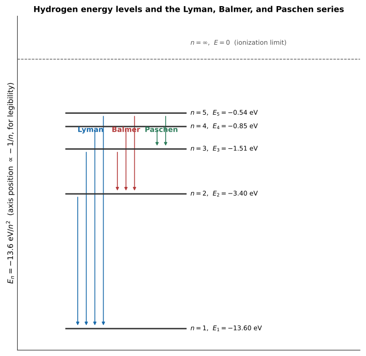
Figure 10.3:Hydrogen energy levels –5 (vertical position compressed for legibility; labels give the real ), with the Lyman, Balmer, and Paschen series drawn as clusters of downward transitions converging on , 2, and 3 respectively. Each series’ shortest-wavelength member is its series limit, reached only as . Computed directly from ; see scripts/figures/.
Worked Example: The Balmer Series and the Visible Spectrum¶
The Rydberg formula is simply rewritten as a wavelength via :
Find (a) the wavelength of , the first (longest-wavelength) line of the Balmer series (), and (b) the Balmer series limit.
(a)
a deep red line — the line used to image glowing hydrogen gas in nebulae and to trace the rotation of spiral galaxies.
(b) As , , so
just past the violet edge of the visible spectrum, in the near ultraviolet. Every Balmer line falls between these two wavelengths, — which is why nearly the whole series, unlike the entirely ultraviolet Lyman series or the entirely infrared Paschen series, is visible to the human eye, and why Johann Balmer found the first four of these lines by curve-fitting alone in 1885, three decades before Bohr’s model — or Schrödinger’s equation — existed to explain them.
Electron Spin¶
By the mid-1920s, several pieces of spectroscopic evidence — most directly, the splitting of atomic beams passing through an inhomogeneous magnetic field — showed that the three quantum numbers do not fully specify an electron’s state. In the Stern–Gerlach experiment (1922), a beam of (electrically neutral) silver atoms was passed through a strongly inhomogeneous magnetic field and allowed to strike a detector screen. A classical magnetic dipole, oriented randomly, should be deflected by an amount depending continuously on its orientation, producing a single smeared-out band on the screen. Instead, the beam split into exactly two discrete spots, symmetric about the undeflected position — direct evidence of space quantization (Chapter 9) applied to a new, previously unsuspected degree of freedom, since the outermost electron in a silver atom happens to be in an -state (, hence zero orbital angular momentum and no orbital magnetic moment to produce any deflection at all), so the observed splitting could not be due to orbital angular momentum.
The resolution, proposed by Samuel Goudsmit and George Uhlenbeck (1925), is that the electron possesses an intrinsic angular momentum, spin, , with no classical counterpart (it is not literally the electron spinning on its axis — such a picture leads to internal-consistency and speed-of-rotation contradictions and should be regarded purely as a suggestive name), quantized exactly as orbital angular momentum is, but with a spin quantum number restricted to the single value :
The two allowed values of — “spin up” and “spin down” — account exactly for the two Stern–Gerlach spots. A complete specification of an electron’s state in hydrogen therefore requires four quantum numbers, , and the count of degenerate states for a given becomes rather than , the factor of 2 from the two spin orientations — a result central to the structure of the periodic table in Chapter 11.
10.3Magnetic Moments and Selection Rules¶
Magnetic Moments¶
Both orbital and spin angular momentum give the electron a magnetic dipole moment, since a circulating (or intrinsically “spinning”) charge behaves as a small current loop. The orbital magnetic moment is
where is the Bohr magneton, a natural unit of atomic magnetic moment. The spin magnetic moment has an analogous form but with an extra numerical factor (the electron’s -factor, , itself a prediction of relativistic quantum theory beyond the scope of the nonrelativistic Schrödinger equation used here):
These magnetic moments are what couple to an external magnetic field in the Stern–Gerlach experiment (producing the observed splitting and deflection) and, coupling to each other and to nuclear magnetic moments, produce the fine and hyperfine splittings observed in high-resolution atomic spectra.
The Stern–Gerlach Force and a Numeric Deflection¶
A uniform magnetic field exerts a torque on a magnetic dipole — producing the Larmor precession pictured in Chapter 9’s precessing-top figure — but exerts zero net force, because the interaction energy does not depend on position when itself does not. Deflecting the beam at all, as Stern and Gerlach needed to do to see anything on their screen, requires a spatially varying (inhomogeneous) field, whose gradient converts the dipole’s orientation into a genuine transverse force:
pushing atoms with one way and the other. Because takes only the two discrete values (from the spin-moment formula above, with and ) rather than a continuum of values, the beam splits into exactly two discrete trajectories instead of spreading into one continuous smear — the direct experimental signature of space quantization that motivated this section.
Worked Example: Beam Splitting in a Stern–Gerlach Magnet¶
A beam of silver atoms () effuses from an oven at , giving a typical beam speed . The beam passes through a magnet of length producing a field gradient , then drifts a further to a detector screen. Find the separation between the two spots.
The force on each atom is
giving a transverse acceleration . While inside the magnet, for a time , each atom acquires a transverse displacement and a transverse velocity ; it then drifts (no further transverse force, but still moving at ) for an additional time , adding . The one-sided deflection is , so the two spin states land
apart on the screen — comfortably resolvable, and the same order of magnitude as the splitting Stern and Gerlach actually measured in 1922 with a weaker gradient over a shorter path, which is what made their two-spot pattern (rather than one smeared band) unambiguous.
The Zeeman Effect¶
Chapter 9 introduced the (normal) Zeeman effect qualitatively: an external field along adds an energy to each otherwise-degenerate sublevel of a given . Including the spin moment as well, the total field-induced shift of a state is
so that adjacent orbital sublevels are separated by exactly . For electric-dipole transitions, the corresponding magnetic quantum-number rule is : the transitions produce the two side components, while produces the central component of the normal Zeeman triplet. Historically, it was the observed splitting pattern (sometimes the simple three-line “normal” Zeeman pattern predicted by alone, but more often a more complicated “anomalous” pattern explainable only once spin and its distinct -factor were included) that provided some of the earliest indirect evidence for electron spin, years before Stern and Gerlach identified its direct mechanical signature.
Worked Example: Zeeman Splitting Frequency in a 1 T Field¶
Estimate the frequency splitting between adjacent sublevels for a hydrogen atom in a field (a typical laboratory electromagnet), and the resulting wavelength shift of the line (, from the worked example above).
(the electron’s Larmor precession frequency in this field). Converting to a wavelength shift via ,
about times smaller than the line’s own wavelength — invisible by eye, but well within reach of a laboratory grating with resolving power (Chapter 5), which is how the Zeeman effect is actually resolved in the lab.
Fine Structure: Spin–Orbit Coupling¶
Even with no external field at all, the energies are not quite the whole story. A useful semiclassical picture is that, in the electron’s rest frame, the orbiting (positively charged) nucleus constitutes a circulating current that produces a magnetic field at the electron’s location. That internal field couples to the electron’s spin magnetic moment, with the necessary relativistic treatment—including Thomas precession—giving the interaction called spin–orbit coupling. Its strength depends on the relative orientation of and (equivalently, on the total angular momentum ). Spin–orbit coupling vanishes for , but the full fine structure also includes relativistic kinetic-energy and Darwin corrections, so -states can receive fine-structure shifts as well. A complete treatment requires relativistic quantum mechanics beyond the nonrelativistic Schrödinger equation used throughout this book. What matters here is the size of the resulting fine-structure correction:
where , the dimensionless fine-structure constant, measures the intrinsic strength of the electromagnetic interaction and sets the size of essentially every relativistic correction in atomic physics. Because , fine structure shifts a level by only a few parts in 105 of itself — far too fine to see with a simple grating, but readily resolved with a high-resolution spectrometer, and the historical reason spectral lines that look perfectly sharp in an introductory demonstration reveal themselves, under sufficient magnification, to be closely spaced multiplets (hence the name, coined for exactly this kind of fine-toothed splitting of what earlier instruments saw as a single line).
Worked Example: Order-of-Magnitude Fine-Structure Splitting¶
Estimate the fine-structure splitting of hydrogen’s level, and compare it to the actual measured splitting of the levels, (equivalently, about ).
within about a factor of four of the measured value — entirely appropriate for an order-of-magnitude estimate that drops the numerical factors (-dependence and other combinatorics supplied only by a full relativistic treatment) while correctly capturing the essential physical scale: fine structure is smaller than the gross level spacing by a factor of , the same small parameter that controls, order by order, essentially every relativistic correction in atomic physics.
The same coupling, applied to the proton’s magnetic moment rather than the electron’s, is the basis of magnetic resonance imaging, and Figure 10.4 is a working model of it. A static field along splits the two spin orientations by , which for a proton in a field falls in the radio band; a transverse radio-frequency field tuned to exactly that frequency drives transitions between them, and the resonance is sharp enough that a deliberate spatial gradient in makes the resonant frequency a map of position. Everything in the sequence — the splitting proportional to , the resonance condition , the return to equilibrium afterwards — is this section’s physics with replaced by the nuclear magneton.
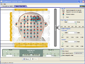
Figure 10.4:Proton spins in a magnetic field: Zeeman splitting, resonant absorption of a radio-frequency photon, and the field gradient that turns the resonance into an image.
Interactive simulation: Simplified MRI
Selection Rules¶
Not every pair of hydrogen energy levels is connected by an observable spectral line. An electron making a transition between stationary states typically does so by emitting or absorbing a single photon, and conservation of angular momentum and parity restricts which transitions can occur via this single-photon (electric dipole) process. The principal orbital selection rule is
and the magnetic quantum number must obey ; the electron’s spin projection is unchanged, . There is no similarly strict restriction on , but the electric-dipole transition must change parity, which the rule already guarantees for hydrogen orbitals. Transitions violating these rules (e.g., , both ) are called forbidden transitions — not absolutely impossible, but strongly suppressed, occurring (if at all) only through much slower, higher-order processes. The selection rules are why, for instance, the observed hydrogen spectral series (Lyman, Balmer, Paschen, etc., corresponding to transitions ending on ) show specific line patterns rather than a line for every conceivable pair of levels.
10.4Summary¶
The radial Schrödinger equation for hydrogen’s Coulomb potential reproduces the Bohr energy levels , but from normalizability of rather than a postulated orbit, and with the ground state having zero orbital angular momentum, unlike Bohr’s model. Normalizability forces the radial series to terminate into a finite polynomial, which fixes to a positive integer and, via ( the radial node count), caps at .
Bohr’s 1913 model reproduced hydrogen’s spectrum numerically from an unjustified orbit postulate, but could not be extended consistently to helium or predict transition rates, and gets the ground state’s angular momentum flatly wrong — failures that motivated the full Schrödinger treatment.
Hydrogenic ions (e.g. , ) follow and : binding energy scales as , orbital size as .
Hydrogen states are labeled by , , ; because depends only on , there are degenerate spatial states per — a special feature of the pure Coulomb potential.
Explicit radial wave functions , , , and the radial probability distributions they generate, show the node count directly; angular nodal structure gives rise to the characteristic , , orbital shapes. The Bohr radius reappears as the most probable electron-nucleus separation in the ground state.
The effective potential shows that only states have nonzero probability density at the nucleus (although the radial probability vanishes there for every state); higher states are held away from the origin by the centrifugal barrier, a penetration effect central to screening in Chapter 11.
The Lyman, Balmer, and Paschen series (transitions ending on ) each converge to a series limit at ; the Rydberg formula gives their wavelengths, with the Balmer series (364.6–) spanning most of the visible range.
The Stern–Gerlach experiment revealed electron spin, an intrinsic angular momentum with quantum number and , doubling the degenerate state count to and requiring four quantum numbers to fully specify a state. The inhomogeneous-field force converts the two spin orientations into two discrete beam deflections.
Orbital and spin angular momentum each produce a magnetic moment, in units of the Bohr magneton ; the spin moment carries an extra -factor . In an external field, the (normal) Zeeman effect shifts sublevels by ; even with no external field, spin–orbit coupling produces fine-structure splitting of order , where is the fine-structure constant.
Single-photon electric-dipole transitions obey , , and , explaining the observed pattern of hydrogen spectral lines.
10.5Problems¶
Solution to Exercise 10.1 #
For , the Rydberg formula gives
At the series limit, , so . Both lines are the leftmost cluster of downward arrows in Figure 10.3, all converging on . Therefore, the first Lyman line is and the limit is ; both are ultraviolet, so the entire series is invisible to the eye.
Solution to Exercise 10.2 #
For , . The allowed sets are ; ; and . Their count is . Including doubles this count to 18. Therefore, the level has nine spatial states and eighteen states when spin is included.
Solution to Exercise 10.3 #
The changes in are: (a) , so and allowed; (b) , so forbidden; (c) , so allowed; and (d) , so allowed. Because no values are specified, this classification asks whether the orbital transition has any allowed magnetic-sublevel components; those components must also satisfy .
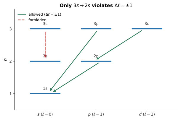
Figure 10.5:Grouping the levels by makes the rule visual: an allowed arrow always moves one column over, while tries to stay in the same column and is forbidden.
Therefore, only is forbidden by the electric-dipole selection rule.
Solution to Exercise 10.4 #
For ,
The largest magnitude of is 2, and (the sign is opposite to that of for an electron). Therefore, the electron has orbital angular momentum and maximum -component magnetic-moment magnitude .
Solution to Exercise 10.5 #
Silver has one unpaired outer electron. An state has , so it has no orbital magnetic moment that could obscure the result; the two-way splitting is therefore due cleanly to spin. Helium’s paired electrons have canceling spin moments. Therefore, silver was ideal because its single outer electron leaves an uncompensated spin moment, whereas helium has no net moment.
Solution to Exercise 10.6 #
Ignoring the positive normalization constant, . Differentiation gives
For , the derivative vanishes at , changing from positive to negative there — exactly the peak of the curve in Figure 10.2. Therefore, the ground-state radial probability is largest at the Bohr radius .
Solution to Exercise 10.7 #
Hydrogenic ionization energy scales as and the most-probable radius as . Thus
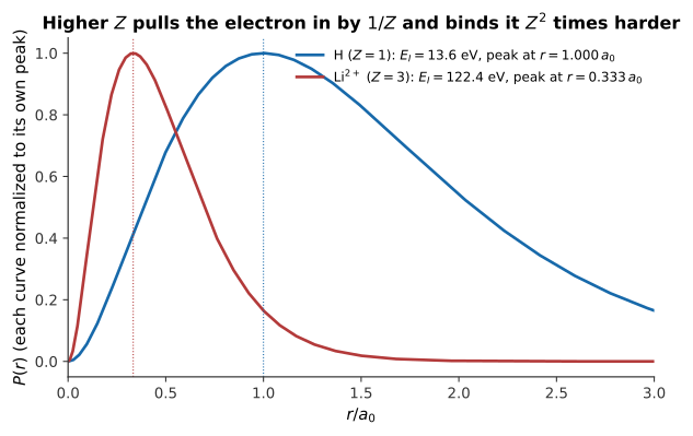
Figure 10.6:Both curves have the same shape, rescaled: replacing with compresses the peak radius by while (not shown to the same vertical scale) the binding energy grows by .
Therefore, has a ionization energy and a most-probable radius: nine times hydrogen’s energy and one-third its radius.
Solution to Exercise 10.8 #
The force magnitude is , so . The magnet time is and the drift time is . One component deflects by
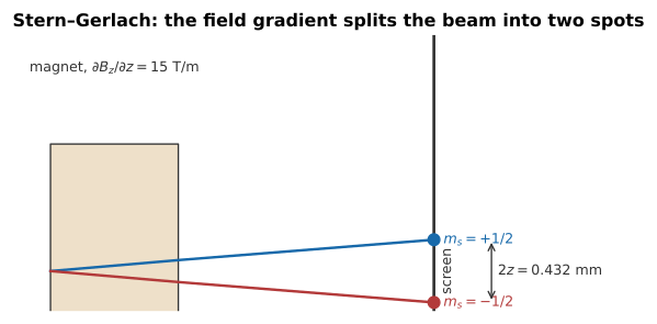
Figure 10.7:The two spin states feel opposite forces inside the magnet, coast in straight lines afterward, and arrive at the screen separated by . (The deflection is exaggerated for visibility; the real displacement is a fraction of a millimeter.)
Therefore, the two opposite spin components are separated by .
Solution to Exercise 10.9 #
Adjacent orbital sublevels differ by , so
Finally .
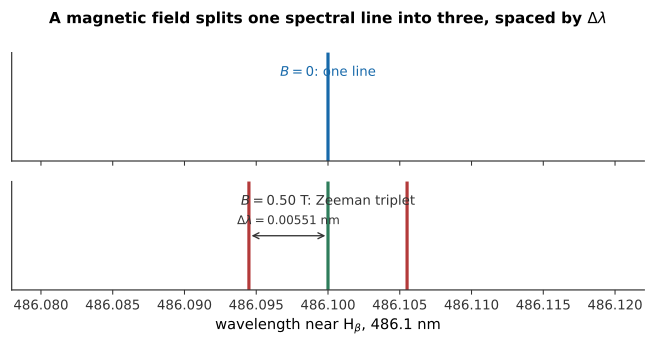
Figure 10.8:The field-free H line becomes a triplet spaced by , one component for each sublevel the upper and lower states split into.
Therefore, the splitting is , , and : the energy and frequency splittings are exactly half the corresponding values (both scale purely with ), but the wavelength shift is not simply half the worked example’s , since it also depends on and ’s wavelength differs from ’s.
Solution to Exercise 10.10 #
For , and . Thus
This is of the estimate because . Therefore, the fine splitting is of order and becomes harder to resolve as rises.