Learning Objectives
By the end of this chapter, you should be able to:
State the de Broglie hypothesis and compute the de Broglie wavelength of a particle.
Explain how the de Broglie hypothesis reinterprets the Bohr model’s angular-momentum quantization condition as a standing-wave requirement.
Describe the Davisson–Germer and G. P. Thomson experiments and explain why they confirm the de Broglie hypothesis, and describe how matter-wave interference has since been extended to atoms and large molecules.
Explain wave–particle duality and complementarity, and describe how “which-path” information destroys interference.
Construct a wave packet as a superposition of waves and relate its spatial and momentum spread; distinguish phase velocity from group velocity and show that group velocity equals particle velocity.
State, derive qualitatively, and apply the Heisenberg uncertainty principle for position–momentum and energy–time.
Use the uncertainty principle to estimate minimum energies and to explain why electrons cannot exist inside a nucleus.
Introduction
Chapter 6 established that light, long understood as a wave, also behaves as a stream of particle-like quanta in its interactions with matter. In 1924, Louis de Broglie proposed the converse: that matter, long understood as composed of particles, should also exhibit wave behavior. This was not an experimental discovery but a bold symmetry argument, made in de Broglie’s doctoral thesis, and it proved correct. This chapter develops the de Broglie hypothesis, the experiments that confirmed it, and its most important consequence: because a particle with a well-defined wavelength is necessarily spread out in space, position and momentum cannot both be known with unlimited precision. That trade-off, the Heisenberg uncertainty principle, is not a statement about the limits of measurement technique but a fundamental feature of nature, and it sets the stage for the wave mechanics developed in Chapter 8.
7.1Matter Waves: de Broglie and Experiment
The de Broglie Hypothesis
Chapter 6 established that a photon carries momentum related to its wavelength by . De Broglie’s proposal was to take this relation, turn it around, and apply it universally: every material particle of momentum has an associated wavelength
now called the de Broglie wavelength. For a nonrelativistic particle of mass and speed , , so ; more generally, for a particle accelerated from rest through a potential difference , gives and hence . Because is so small, the de Broglie wavelength of ordinary macroscopic objects is utterly negligible — a mass moving at has , far too small to produce any observable wave effect — which is why matter waves went unnoticed until physicists deliberately looked for them in systems where is not negligible, such as low-energy electrons, whose small mass makes comparable to atomic and crystal-lattice spacings for accessible kinetic energies.
Worked Example: De Broglie Wavelength of an Accelerated Electron
An electron is accelerated from rest through a potential difference of , a typical value in early electron-diffraction experiments. Its nonrelativistic momentum is
so the de Broglie wavelength is
This convenient combination is often written for nonrelativistic electrons. The result, , is comparable to the spacing between atomic planes in a crystal (–) — exactly the condition needed for the crystal to act as a diffraction grating for the electrons, as the next section describes.
A Consistency Check: The Relativistic Origin of 
De Broglie did not simply guess ; he arrived at it by demanding consistency between the photon relations of Chapter 6 and the relativistic energy–momentum relation of Chapter 3. A wave of frequency and phase speed has wavelength . Associating a particle of energy with a wave of frequency (the Planck–Einstein relation, extended by hypothesis to matter) and demanding that the resulting phase velocity be consistent with the particle’s momentum via (the relativistic relation between energy, momentum, and velocity established in Chapter 3) leads, after eliminating and in favor of , , and the particle’s actual velocity , directly to — the same relation obtained by simply carrying the photon formula over to matter, but now derived from relativistic energy–momentum consistency rather than asserted by analogy alone. This is one reason de Broglie’s hypothesis, though speculative, was taken seriously immediately: it was not an arbitrary guess but the unique relation consistent with treating matter and light on the same relativistic footing.
The Davisson–Germer and G. P. Thomson Experiments
Direct confirmation came in 1927, when Clinton Davisson and Lester Germer, studying electron scattering from a nickel crystal (originally for an unrelated purpose), observed that the intensity of electrons scattered from the crystal surface showed sharp maxima at specific angles, depending on the electrons’ kinetic energy — exactly the pattern expected from diffraction of a wave by the regularly spaced planes of atoms in the crystal, analogous to X-ray diffraction from a crystal lattice (Bragg diffraction). Measuring the angles of the diffraction maxima and applying the same diffraction condition used for X-rays,
(with the crystal’s known interplanar spacing and measured from the planes) allowed Davisson and Germer to extract an experimental wavelength for the electrons — and it agreed, to good precision, with the de Broglie wavelength computed from the electrons’ known kinetic energy.
The experiment is reconstructed in Figure 7.1, where both sides of are under control: the electron gun’s accelerating voltage, which fixes and hence , and the spacing of the target atoms, which fixes . Raising the voltage shortens the wavelength and pulls the scattering maxima to smaller angles; widening the atomic spacing pushes them back out. Neither response is available to a stream of particles bouncing off a surface, and observing both is what settled the question.
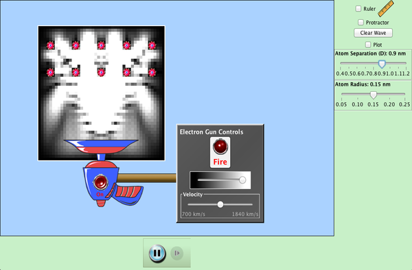
Figure 7.1:Electrons scattering from a crystal surface, with the beam energy and the atomic spacing under control. What is drawn is the electron’s wave; where it is detected is a single point.
Interactive simulation: Davisson–Germer: Electron Diffraction
That same year, working independently in Britain, George Paget Thomson fired higher-energy electrons through thin polycrystalline metal foils and observed concentric diffraction rings on a photographic plate — the electron analog of the ring patterns produced by X-ray diffraction through a powdered crystalline sample — providing an independent confirmation using a completely different experimental geometry. Thomson’s result carries a particular irony: his father, J. J. Thomson, had won the 1906 Nobel Prize for discovering the electron and demonstrating that it is a particle with a definite charge-to-mass ratio; the son shared the 1937 Nobel Prize (with Davisson) for demonstrating that the very same particle also behaves as a wave — both experiments correct, neither in conflict with the other, once wave–particle duality is properly understood.
Electrons, unambiguously particles in every other respect (they have definite charge and mass, and leave localized tracks and point-like impacts on a detector), diffract like waves when their de Broglie wavelength is comparable to the spacing of the diffracting structure. The effect has since been confirmed for neutrons, atoms, and — in experiments beginning in the late 1990s — even large molecules: neutron diffraction is now a standard tool for probing crystal and magnetic structure (complementing X-ray diffraction, since neutrons, being uncharged, scatter primarily from nuclei rather than electron clouds), and a landmark 1999 experiment by Arndt, Zeilinger, and collaborators observed diffraction of “buckyball” molecules — each containing 60 carbon atoms, with a mass roughly 106 times that of a single electron — through a microfabricated grating, with a measured de Broglie wavelength of only a few picometers, far smaller than the molecule itself, yet still large enough to produce a measurable diffraction pattern. Matter-wave interference is not a special property of electrons; it is a universal feature of quantum objects, observable whenever a system can be prepared with a de Broglie wavelength comparable to some accessible length scale. The same phenomenon is the operating principle of the electron microscope, whose resolution — set by the wavelength of the imaging “light,” per ordinary diffraction limits (Chapter 5) — can be far finer than any visible-light microscope because electron de Broglie wavelengths, as the worked example above shows, can be made far shorter than visible wavelengths simply by choosing a sufficiently large accelerating voltage.
Neutron Interferometry
Because neutrons are electrically neutral, they can be split into two coherent beams and recombined using neutron interferometers built from a single, precisely machined crystal of silicon, without the beam-steering complications that an electron’s charge would introduce in a magnetic or electric field. A landmark 1975 experiment by Colella, Overhauser, and Werner (the “COW experiment”) used exactly this technique to observe a measurable phase shift between the two arms of a neutron interferometer when one arm was raised slightly in the Earth’s gravitational field relative to the other — a direct demonstration that a quantum matter wave, not merely a mathematical bookkeeping device, is affected by gravity precisely as its de Broglie wavelength and the classical gravitational potential energy predict. Neutron interferometry has since been used to test the sign and magnitude of gravitational, and even rotational (Sagnac), phase shifts on matter waves with high precision, extending the reach of wave–particle duality from crystal diffraction to macroscopic-scale sensitivity to gravity itself.
The Bohr Quantization Condition Revisited
The de Broglie hypothesis retroactively explains a feature of the 1913 Bohr model of the hydrogen atom (developed further in Chapter 10) that Bohr himself had simply postulated without justification: that an orbiting electron’s angular momentum is quantized in integer multiples of , . If the electron in a circular orbit of radius is described by a de Broglie wave of wavelength , that wave can only form a consistent, single-valued standing pattern around the orbit if the orbit’s circumference contains a whole number of wavelengths,
since otherwise the wave would interfere destructively with itself on successive trips around the loop and no stable pattern could persist. Rearranging, — exactly Bohr’s angular-momentum quantization condition, , now derived (rather than assumed) from the requirement that an electron’s matter wave close consistently on itself. This does not yet constitute a full theory (that requires the Schrödinger equation of Chapters 8–9, applied to the hydrogen atom in Chapter 10), but it shows that de Broglie’s hypothesis was not an isolated curiosity: it directly explains why atomic angular momentum comes only in discrete multiples of , years before Schrödinger’s wave equation made the connection rigorous.
Quantization by a closure condition is not a quantum idea, and it is easier to trust once it has been seen somewhere unmysterious. Figure 7.2 drives a column of air and sweeps the frequency: almost every frequency produces nothing, and at a discrete set of them the tube suddenly resonates, because only there does the wave returning from the far end arrive back in step with itself. Nothing is quantized about air. What is discrete is the set of wavelengths that a boundary condition permits — an integer count fitting into the available length — and de Broglie’s contribution was to notice that an electron’s wave going around an orbit is subject to a closure condition of exactly the same kind.
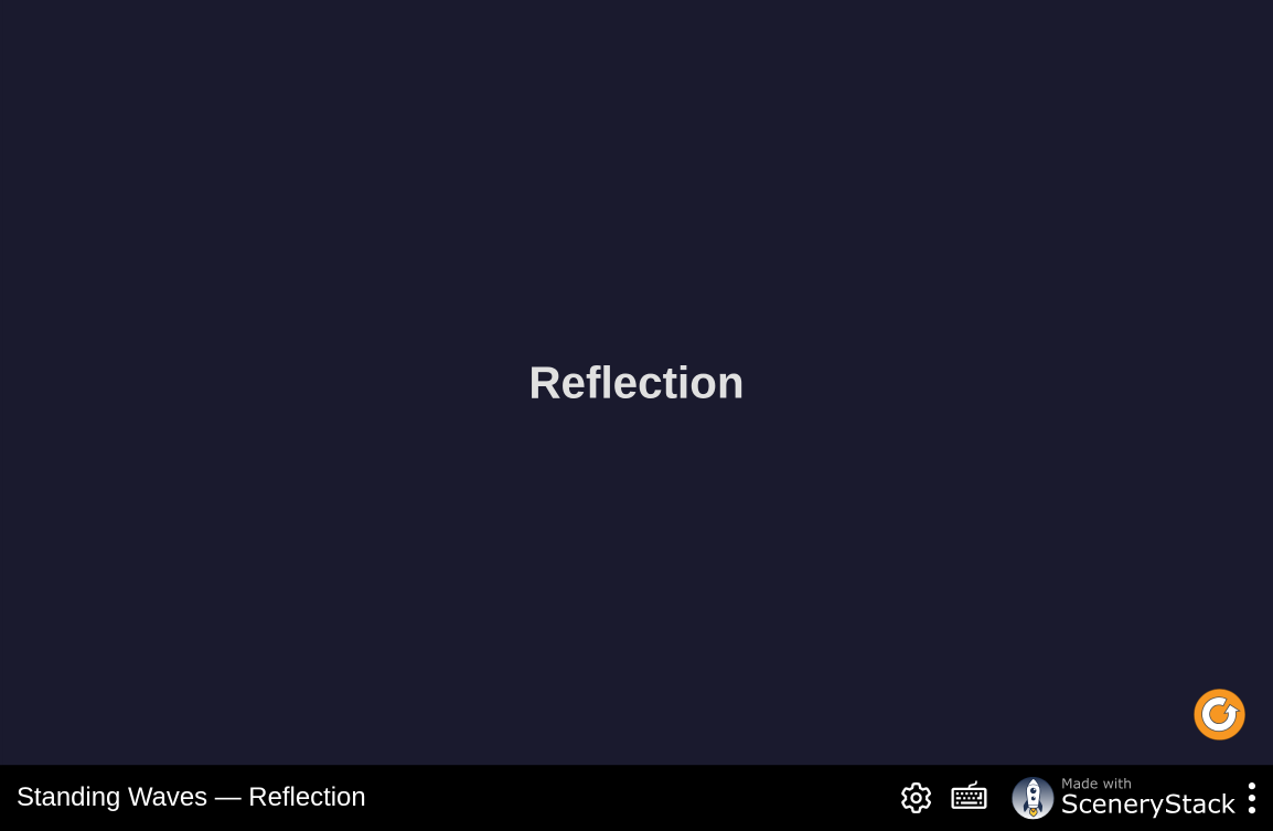
Figure 7.2:Standing waves in a pipe. Sweep the drive frequency and the response is a set of sharp resonances at which a whole number of half-wavelengths fits between the ends; between them, the returning wave arrives out of step and cancels itself. The Bohr condition is the same statement for a wave that closes on a loop instead of between two ends.
Interactive simulation: Standing Waves
Worked Example: Checking the Standing-Wave Condition for Hydrogen’s Ground State
The Bohr model (developed further in Chapter 10) gives the electron in hydrogen’s orbit a radius (the Bohr radius) and an orbital speed . Its de Broglie wavelength is
while the orbit’s circumference is — the two agree to three significant figures, exactly confirming the standing-wave condition for : the ground-state orbit’s circumference is precisely one de Broglie wavelength.
7.2Wave–Particle Duality and Wave Packets
Wave–Particle Duality
The picture that emerges from Chapters 6 and 7 together is symmetric: light, ordinarily described as a wave, exhibits particle-like behavior (photoelectric effect, Compton scattering); matter, ordinarily described as particles, exhibits wave-like behavior (electron diffraction). Neither description is simply “wrong” and replaced by the other; rather, both light and matter possess both wave and particle aspects, and which aspect is manifest depends on the experiment performed. This is wave–particle duality, and its sharpest expression is Niels Bohr’s principle of complementarity: the wave and particle descriptions are both necessary for a complete account of quantum behavior, both cannot be exhibited in full simultaneously by the same experimental arrangement, and neither alone is sufficient.
The double-slit experiment (Chapter 4) makes this concrete. Even when electrons (or photons) are sent through the apparatus one at a time — far too infrequently for any two particles to interact or “interfere with each other” in transit — the individual, localized detection events recorded on a screen accumulate, after many particles, into the same interference fringe pattern predicted for a wave. Each particle arrives as a single, point-like click, exactly as a particle should; yet the statistical distribution of many such clicks builds up the wave-interference pattern, meaning each individual particle’s behavior is governed by the same wave mathematics used for light, even though no two particles are present in the apparatus at once to “interfere” with each other in any classical sense. This experiment has been performed with electrons (originally by Claus Jönsson in 1961, and in a particularly clean single-particle-at-a-time form by Akira Tonomura and collaborators in 1989) and confirms the interference pattern exactly as quantum mechanics predicts.
That accumulation is the thing to watch, and it is what Figure 7.3 reproduces. Fire particles one at a time and the screen records isolated, point-like hits in what looks at first like a random scatter; leave it running and the fringes emerge from the statistics of hits that were never anything but individual. The simulation also carries the which-path apparatus discussed next: a detector placed in the path of the wave function collapses it on each measurement, and the fringes go with it, while the individual hits go on looking exactly the same.
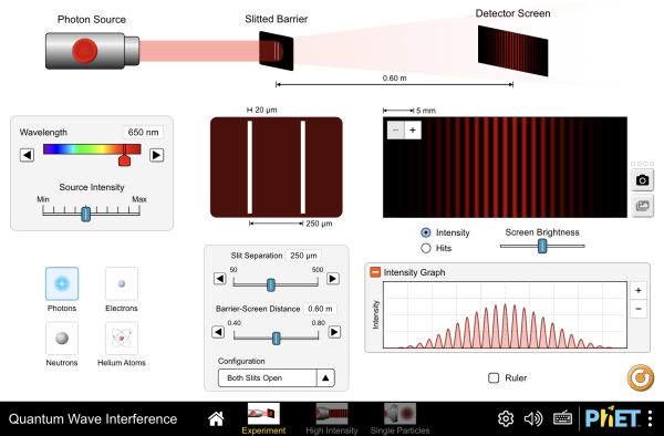
Figure 7.3:Single particles sent through a double slit, one at a time, with the detection screen accumulating hits. The wave function is displayed alongside the record of impacts: one object, propagating as a wave and detected as a particle.
Interactive simulation: Quantum Wave Interference
Crucially, if a measurement is added to the apparatus that determines which slit each particle actually passed through — “which-path” information — the interference pattern disappears entirely, replaced by the simple sum of the two single-slit patterns, exactly as if the particles were classical objects going through one slit or the other. The loss of interference is not limited to a literal momentum kick: a which-path detector can also mark the alternatives by entangling the particle with another degree of freedom, such as polarization or an internal detector state. Once those alternatives are distinguishable even in principle, their amplitudes no longer combine to produce interference; an uncertainty-principle momentum disturbance is one important realization, not the general explanation. It is tempting, but incorrect, to imagine that a photon or electron is “really” a tiny wave packet that sometimes behaves like a particle, or “really” a tiny particle that sometimes behaves like a wave; the two descriptions are complementary, and a full account of quantum behavior (developed starting in Chapter 8) requires a mathematical object — the wave function — that reduces to particle-like or wave-like predictions depending on what is measured, without being fully captured by either classical picture on its own.
Delayed Choice and the Quantum Eraser
A particularly striking variant, proposed by John Wheeler in 1978 and since realized experimentally, asks whether the decision to measure which-path information can be postponed until after a particle has, in some naive classical sense, “already passed” through the slits. In a delayed-choice experiment, the choice of whether to record which-path information (destroying the interference pattern) or to erase it before the particle is detected (restoring the interference pattern) is made only at the very last possible moment — in some realizations, only after the particle has already traversed the region of the slits. Experiments of this kind confirm quantum mechanics’ prediction exactly: interference reappears in the appropriate measurement outcomes whenever the alternatives are made indistinguishable, regardless of when in the experiment that choice is made. A related arrangement, the quantum eraser, first correlates each particle with a “marker” that could reveal which path it took, then either reads that marker (destroying the interference pattern in the corresponding subset of detection events) or measures it in a basis that erases the path distinction (revealing interference only in appropriately sorted subsets). Neither experiment allows sending a signal backward in time or violates causality. If the marker result is ignored, the unconditional detection pattern remains interference-free; the fringes in a sorted subset become visible only after the corresponding marker records are compared. These results reinforce the same lesson as the ordinary double-slit experiment: a quantum system does not carry a hidden, predetermined trajectory waiting to be revealed, and complementarity is a statement about what information can coexist, not merely about the limits of measurement technology.
Wave Packets
To describe a localized particle in wave language, a single wave of definite wavelength — which by its nature extends infinitely in space with constant amplitude — is not adequate, since it corresponds to a perfectly definite momentum but gives no information about where the particle is. A localized particle is instead represented by a wave packet: a superposition of many waves of slightly different wavelength (equivalently, different wave number ), chosen so that they interfere constructively in some limited region and destructively (cancel) elsewhere. The mathematics of superposition (the same mathematics used for beats and Fourier synthesis of waveforms) requires that a packet localized to a narrow spatial region necessarily be built from a broad range of wave numbers , and vice versa; the two spreads are inversely related, roughly
a purely mathematical fact about waves, true for sound pulses and water-wave packets just as much as for matter waves, with no quantum content yet.
The trade-off can be watched directly. Figure 7.4 builds a packet out of harmonic components whose amplitudes follow an adjustable envelope, and prints both widths as you work: narrow the spread of contributing wave numbers and the packet in stretches out toward the infinite sinusoid of definite momentum; widen and the packet contracts toward a spike, with the panel reporting throughout. Switching the display from a function of space to a function of time turns the same relation into the energy–time form used later in this section.
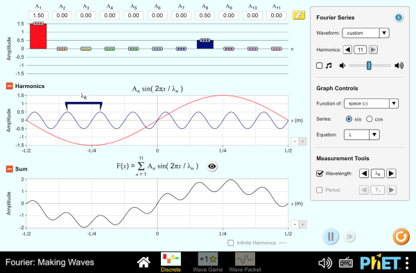
Figure 7.4:A wave packet and the Fourier components that build it, with the width in and the width in both displayed. Their product cannot be reduced: this is the classical wave theorem that becomes the uncertainty principle once is imposed.
Interactive simulation: Fourier: Making Waves
Quantum mechanics enters when this relation is combined with the de Broglie relation (where ), converting spread in wave number into spread in momentum, , and giving
Phase Velocity and Group Velocity
A wave packet built from components of angular frequency spread over a narrow range of can be shown, by adding two nearby component waves and , to have an overall envelope that moves at the group velocity
which is, in general, different from the phase velocity at which the individual wave crests inside the envelope move.
For a nonrelativistic free particle, the de Broglie relations and , combined with the nonrelativistic kinetic-energy relation , give
so that
exactly the classical particle velocity — the wave packet’s envelope, the physically observable, localized “blob” of probability, moves at precisely the speed a classical particle with the same momentum would have. The phase velocity, by contrast, is , exactly half the particle’s actual speed: the individual crests inside the packet move at a different, less physically meaningful speed than the envelope itself, a reminder that it is the group velocity, not the phase velocity, that corresponds to the motion of the particle (and, for a light pulse in an ordinary, weakly dispersive medium, that closely tracks the speed at which energy and information travel — the two velocities can part ways near a strong absorption line, but that subtlety does not arise here).
Deriving the envelope speed from two superposed waves
The group-velocity formula can be seen directly by adding just two component waves of equal amplitude, wave numbers , and angular frequencies :
Using the sum-to-product identity with and the two bracketed phases gives
The first factor is a rapidly oscillating carrier wave moving at the phase velocity ; the second factor is a slowly varying envelope — the “beat” pattern familiar from superposing two close sound frequencies — whose crests (where the cosine argument is constant) move at speed . Adding more and more component waves in a narrow band around sharpens this beat pattern into a single, well-localized wave packet, and in the limit the envelope speed becomes exactly , the group velocity used in the main text.
Wave Packet Spreading
The nonrelativistic dispersion relation in Equation (7.10) is not linear in (unlike the dispersion relation for light in vacuum), which has a further consequence beyond fixing the group velocity: different Fourier components of a wave packet, corresponding to different momenta, travel at slightly different group velocities , since a component with larger (larger momentum) simply moves faster. A packet initially localized to a narrow width therefore does not maintain its shape as it propagates; because it necessarily contains a spread of wave numbers (the same uncertainty relation used earlier in this section), and each component travels at a slightly different speed, the packet’s spatial width grows with time — it spreads. A careful calculation shows the spreading time scale is of order : a light particle (small ) confined to a very small initial region (small ) spreads apart quickly, while a macroscopic object’s wave packet spreads on a time scale so astronomically long that the effect is entirely unobservable — one more reason, alongside the negligible de Broglie wavelength itself, that ordinary macroscopic objects appear to follow sharp, well-defined classical trajectories rather than visibly diffusing.
7.3The Heisenberg Uncertainty Principle
Werner Heisenberg (1927) elevated the wave-packet relation above to a fundamental principle governing all quantum systems, stated precisely as
where and are, more precisely, statistical spreads (standard deviations) in simultaneous measurements of position and momentum made on identically prepared systems. The Heisenberg uncertainty principle states that these two spreads cannot both be made arbitrarily small: the more precisely a particle’s position is known, the less precisely its momentum can be known, and conversely. This is not a statement about the clumsiness of measuring instruments, correctable in principle by better technology — it is a consequence of the wave nature of matter itself, as the wave-packet argument above shows: a particle simply does not possess simultaneously well-defined position and momentum, in the same sense that a wave pulse of well-defined wavelength cannot also be localized to a point.
An analogous relation holds between energy and time,
where characterizes the time available to measure (or the lifetime of a state with) energy spread . This relation, for instance, explains why an unstable state with a short lifetime (such as an excited atomic state, or an unstable particle) necessarily has an intrinsic spread, or “width,” in its energy — and correspondingly in the frequency/wavelength of radiation it emits — that grows as its lifetime shrinks.
Stripped of , this is a theorem about signals rather than about quantum mechanics, and it applies to any wave one cares to measure — including the sound of one’s own voice. Figure 7.5 runs a live spectrum of whatever the microphone hears: a sustained vowel, going on for a long , resolves into sharp harmonic lines with small , while a clipped consonant lasting a few milliseconds has no sharp lines at all, only a broad smear across the spectrum. No better microphone would fix this. A short signal does not have a well-defined frequency, exactly as a short-lived excited state does not have a well-defined energy.
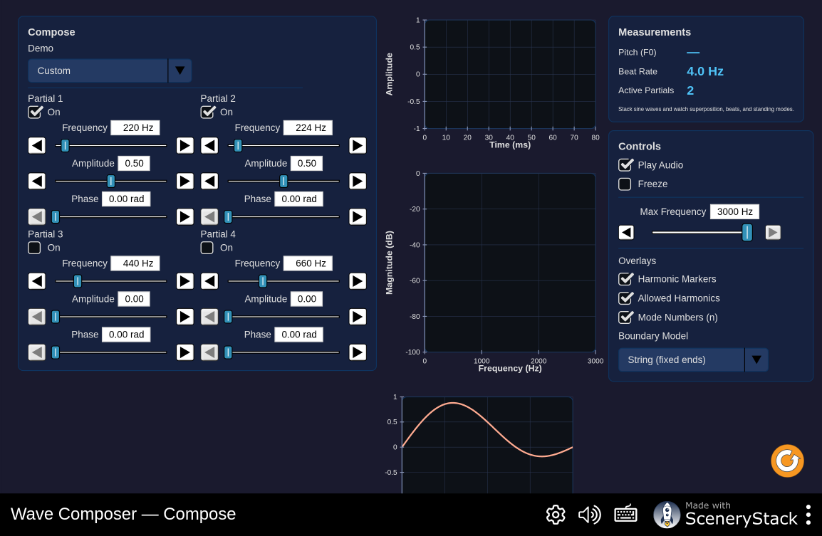
Figure 7.5:Real-time spectrum analysis of a microphone signal. The duration of a sound and the sharpness of its spectrum trade off against each other, which is with the removed and the quantum mechanics along with it.
Interactive simulation: Wave Composer
Worked Example: Confining an Electron in a Nucleus
Could an electron exist bound inside an atomic nucleus, of radius ? If so, the position uncertainty could be no larger than , and the uncertainty principle then requires a momentum uncertainty of at least
Converting to an energy via the (relativistic, since this momentum turns out to be large) relation for : . An electron confined to nuclear dimensions would need kinetic energy of tens of MeV — far larger than the few-MeV binding energies available in nuclei (Chapter 13) — so such an electron could not remain bound; this is one of the historical arguments (alongside others involving nuclear spin and magnetic moment) that electrons are not constituents of the nucleus, correctly anticipating that beta decay (Chapter 13) must create an electron at the moment of decay rather than releasing one that was previously confined inside.
Worked Example: The Scale of Atomic Energies
The uncertainty principle also correctly predicts the order of magnitude of atomic binding energies, without needing to solve the Schrödinger equation at all. An electron confined to an atom of radius (the Bohr radius, derived properly in Chapter 10) has, by the same reasoning as above, a minimum momentum uncertainty
Since this is small enough that the electron remains nonrelativistic, its kinetic energy is — the right order of magnitude for atomic binding and ionization energies (a few to a few tens of eV), even though the precise numerical value requires the full machinery of Chapters 9–10. This is a recurring pattern in quantum mechanics: the uncertainty principle alone, applied as an order-of-magnitude estimate, correctly anticipates the characteristic energy scale of a confined system, well before an exact calculation is carried out.
7.4Summary
The de Broglie hypothesis assigns every particle of momentum a wavelength , extending the photon relation of Chapter 6 to all matter, and for an electron accelerated through voltage gives .
Requiring an electron’s de Broglie wave to form a consistent standing pattern around a circular orbit, , reproduces the Bohr model’s angular-momentum quantization , previously an unexplained postulate.
The Davisson–Germer and G. P. Thomson experiments confirmed matter waves directly: electrons diffract from a crystal lattice with a wavelength matching , exactly as X-rays do; matter-wave interference has since been observed for neutrons, atoms, and large molecules such as .
Wave–particle duality and Bohr’s complementarity principle: light and matter both show wave and particle behavior; which is manifest depends on the experiment (as the single-particle double-slit experiment and the loss of fringes upon acquiring which-path information both show), and neither classical picture alone is complete.
A localized particle is represented by a wave packet, a superposition of waves over a range of wave numbers ; its envelope moves at the group velocity , which equals the particle’s classical velocity, distinct from the phase velocity of the individual wave crests.
The Heisenberg uncertainty principle, (and analogously ), is a fundamental limit on the simultaneous precision of conjugate quantities, rooted in the wave nature of matter, not a limitation of measuring instruments, and correctly predicts the order of magnitude of confinement energies from nuclear to atomic scales.
7.5Problems
Solution to Exercise 7.1 #
For nonrelativistic particles, . For electrons, . For a proton, . For the baseball,
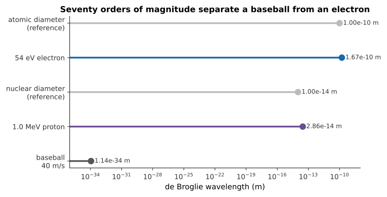
Figure 7.6:Seventy orders of magnitude separate the baseball’s wavelength from the electron’s. Only the electron’s wavelength is comparable to a natural length scale (here, atomic spacing) and can therefore diffract observably.
Therefore, electron waves can diffract from atomic crystal planes, proton waves need nuclear-scale structure, and the baseball wavelength is far too small to observe diffraction.
Solution to Exercise 7.2 #
The electron wavelength from Problem 1 is . First-order Bragg diffraction gives
Therefore, the observed Davisson--Germer maximum corresponds to an effective nickel-plane spacing of under this Bragg-angle convention.
Solution to Exercise 7.3 #
From ,
Therefore, electrons require an accelerating voltage of about to have a de Broglie wavelength.
Solution to Exercise 7.4 #
The thermal energy is . Then
Therefore, room-temperature neutrons have about energy and wavelength, comparable to interatomic spacings and ideal for crystal diffraction.
Solution to Exercise 7.5 #
The molecular momentum is . Thus
The grating period is much larger than this wavelength, but diffraction angles can still be measured and the molecule’s center-of-mass wave can interfere. Therefore, has a few-picometer de Broglie wavelength and can diffract from a nanostructured grating despite being physically larger than its wavelength.
Solution to Exercise 7.6 #
The standing-wave condition is . For , : exactly one de Broglie wavelength fits around the orbit, as shown in Figure 7.7. A shorter circumference would not close in phase, and the one-wavelength state has the smallest allowed momentum and kinetic energy.
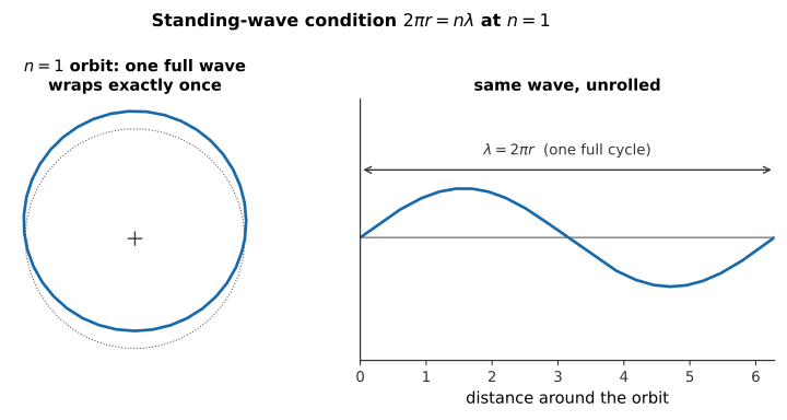
Figure 7.7:Left: the matter wave, wrapped around the orbit, closes on itself after exactly one wavelength. Right: the same wave unrolled into a line, showing directly.
Therefore, the Bohr ground orbit corresponds to the lowest closed standing matter wave.
Solution to Exercise 7.7 #
Taking the confinement width to be the full nuclear diameter, (rather than the radius, as in the electron-in-a-nucleus worked example above — either choice only shifts the order-of-magnitude estimate by a factor of a few) gives the uncertainty-principle lower bound
Here is much smaller than the proton rest energy , so the nonrelativistic estimate is adequate. The corresponding minimum kinetic-energy scale is
The strict uncertainty-principle estimate is therefore a lower bound of roughly , below the several-MeV nuclear binding-energy scale. A particle-in-a-box estimate uses the stronger boundary-condition scale and gives a characteristic ground-state energy of order for , illustrating why the numerical result depends on the confinement geometry; the uncertainty estimate by itself should not be presented as a several-MeV requirement.
Solution to Exercise 7.8 #
Using the common order-of-magnitude convention ,
Since , , giving .
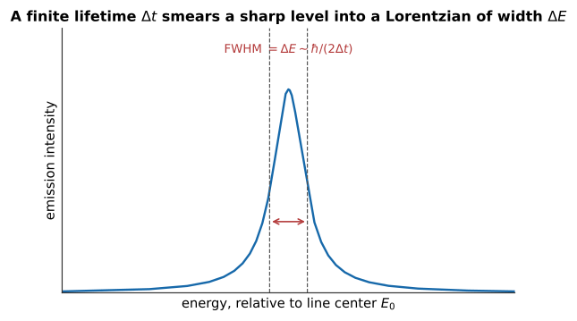
Figure 7.8:A finite-lifetime state cannot have a perfectly sharp energy: the emitted line has a Lorentzian shape whose width is set by .
Therefore, the lifetime implies an energy-spread estimate of about or in wavelength. The precise linewidth and its numerical factor depend on the line-shape and width convention; the uncertainty relation fixes the scale rather than a universal FWHM.
Solution to Exercise 7.9 #
At the first minimum, . Thus
With , . Therefore, single-slit diffraction gives the same position--momentum uncertainty scale required by the uncertainty principle.
Solution to Exercise 7.10 #
For an infinite lifetime, , so the uncertainty lower bound tends to zero. An unstable state has finite lifetime and therefore nonzero energy width. Therefore, stable particles can have sharp rest energies, while unstable particles must be described by both a central mass and a finite decay width.
Solution to Exercise 7.11 #
Differentiate directly:
Therefore, the nonrelativistic matter-wave group velocity equals the particle velocity.
Solution to Exercise 7.12 #
With and ,
The relativistic momentum and energy relations give the same identity . Therefore, the group velocity of a relativistic matter wave is exactly the particle’s physical velocity .
Solution to Exercise 7.13 #
For confinement to , use the same uncertainty estimate as in the worked example, . Then
The atomic-scale worked example used the actual Bohr radius, , as its confinement length, giving . The quantum dot’s confinement length is therefore about times larger, so its confinement energy should be smaller by roughly — consistent with .
For comparison, a one-dimensional infinite-well model gives , a more representative characteristic scale for that geometry. The numerical factor depends on the confinement model, but the scaling — and the much smaller energy than at atomic dimensions — does not.
Solution to Exercise 7.14 #
Determining a slit position to uncertainty gives a transverse momentum spread of at least , or of order when only the diffraction scale is required. This corresponds to an angular spread of order ; for the usual geometry , it is at least comparable to the fringe angle and washes out the fringes. More generally, the detector can destroy interference by entangling the particle with a path marker without a substantial momentum kick: the essential condition is that the two paths become distinguishable, not that every which-path measurement impart the same mechanical disturbance.
Solution to Exercise 7.15 #
For a nonrelativistic free particle, phase velocity is , while the wave packet and all information move at . Individual phase crests are not localized objects and cannot carry a signal. Figure 7.10 shows the same story in the relativistic setting of Problem 19, where the gap between the two velocities is even more dramatic. Therefore, the phase velocity is not an observable propagation speed, so its difference from the group velocity is not paradoxical.
Solution to Exercise 7.16 #
For the electron,
For the dust grain, .
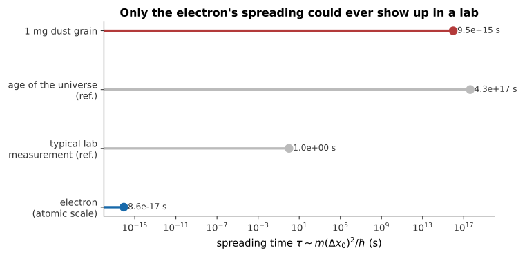
Figure 7.9:The electron’s wavepacket spreads in a fraction of a femtosecond, while the dust grain’s spreading time dwarfs even the age of the universe; only the electron’s spreading could ever appear in a real measurement.
Therefore, electron spreading is extremely rapid, whereas dust-grain spreading is unobservable during a seconds-long laboratory measurement.
Solution to Exercise 7.17 #
Without consulting the marker result, detections in any one output channel form an ordinary interference-free mixture; no observer can tell whether a later eraser choice was made. Interference reappears only after sorting the already-recorded events into correlated subensembles using classical information from the marker/eraser measurement. Therefore, quantum erasure changes conditional correlations, not past detection outcomes, and cannot transmit information backward in time.
Solution to Exercise 7.18 #
Waves reflecting from successive crystal planes differ in total path by : one extra segment on the way in and one on the way out. They reinforce only when this difference is an integer number of wavelengths, ; otherwise their phases cancel in the sum. This is directly analogous to an atomic orbit, where a matter wave survives only when its circumference contains an integer number of wavelengths. Therefore, a diffraction maximum is a standing-wave condition imposed across the periodic crystal lattice.
Solution to Exercise 7.19 #
From and ,
Combining with gives , so .
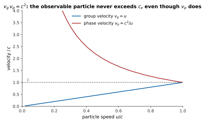
Figure 7.10: never exceeds , while exceeds everywhere except at itself — yet their product is fixed at , and only carries the particle or any information.
This can exceed because phase velocity carries neither a particle nor usable information; the group velocity remains . Therefore, superluminal phase velocity does not violate relativity.
Solution to Exercise 7.20 #
Raising a neutron increases its gravitational potential energy and decreases its kinetic energy by the same small amount. Its momentum therefore decreases and its de Broglie wavelength increases slightly; over a finite path this changes the accumulated phase . Therefore, paths at different heights acquire a measurable relative gravitational phase shift even though the energy change is very small.