Learning Objectives
By the end of this chapter, you should be able to:
Describe light as an electromagnetic wave, relate its wavelength, frequency, and speed, and explain why detectors measure time-averaged intensity rather than the instantaneous field.
Explain why interference and diffraction are invisible in everyday life, using the dimensionless ratio and the correspondence between wave optics and ray optics.
State Huygens’s principle and use it to explain how a wavefront propagates and spreads after an aperture.
Convert a path length difference into a phase difference, and use the result to decide whether two overlapping waves interfere constructively or destructively.
Derive the path-difference conditions for Young’s double-slit experiment, and calculate fringe angles, fringe positions, fringe spacing, and the highest observable order.
Explain why two independent light sources do not produce a stable interference pattern; distinguish temporal from spatial coherence, and estimate coherence length from a source’s spectral width.
Derive the two-slit intensity pattern by phasor addition, show that the central maximum is four times a single slit’s intensity, and explain why this does not violate energy conservation.
Generalize the phasor method to equally spaced, idealized slits, and explain why the principal maxima sharpen as and brighten as .
Apply the thin-film interference conditions, correctly counting the phase shift on reflection from a higher-index medium, to soap films, antireflection coatings, air wedges, and Newton’s rings.
Describe the operation of the Michelson interferometer, convert a mirror displacement into a fringe count, and connect the instrument to the Michelson–Morley experiment of Chapter 1.
Introduction
Chapters 1–3 built special relativity from a single empirical fact: every inertial observer measures the same speed for light. That argument treated light purely as a signal, without asking what, physically, is doing the propagating. Maxwell’s equations answer that question: light is an electromagnetic wave — a self-sustaining, traveling disturbance of the electric and magnetic fields. If that is right, then light must do what every other wave does. It must interfere: two overlapping light waves must be able to reinforce each other in some places and cancel each other in others. And it must diffract: it must bend around obstacles and spread out after passing through an aperture, instead of casting perfectly sharp geometric shadows.
Neither effect is part of ordinary experience. Shadows do look sharp. Light does seem to travel in straight lines. Two flashlights shone on the same wall produce a brighter patch, not a striped one. For most of the seventeenth and eighteenth centuries this was taken as decisive: Newton championed a corpuscular theory, in which light is a stream of tiny particles, and his enormous authority kept the wave theory of his contemporary Christiaan Huygens in the minority for over a century. A large part of this chapter’s job is to explain why the wave effects hide so effectively — the answer, worked out below, is that the wavelength of visible light is a few hundred nanometers, some three orders of magnitude below the smallest object you handle in a day and six or more below a doorway — and then to show what happens when you shrink the apparatus until they can no longer hide.
Thomas Young did exactly that in 1801. He passed light from a single source through two closely spaced slits and found, on a distant screen, not two bright bands but a whole series of alternating bright and dark fringes. There is no way to get dark bands by adding light to light in a particle picture: two streams of corpuscles cannot cancel. In a wave picture the explanation is immediate, quantitative, and gives the wavelength of the light as a bonus. This chapter develops that treatment carefully, and the next takes up the closely related phenomenon of diffraction. Together they put the wave nature of light on the same firm experimental footing that Chapters 1–3 gave to the constancy of its speed — which makes it all the more startling when Chapter 6 shows that light also behaves as a stream of particle-like quanta, and that Newton was not simply wrong.
4.1Waves, Huygens’s Principle, and Superposition
Light as an Electromagnetic Wave
Everything in this chapter follows from one picture of what light is, so it is worth stating carefully before using it.
A monochromatic (single-wavelength) light wave traveling in the direction consists of an electric field oscillating in a direction perpendicular to ,
accompanied by a magnetic field perpendicular to both. Here is the amplitude, is the wave number, is the angular frequency, and is a constant that fixes where in its cycle the wave happens to be at , . The quantity in parentheses is the phase. Wavelength, frequency, and speed are linked in the usual way,
Three consequences of this description are used constantly below.
Detectors measure intensity, not field. The intensity — the power per unit area carried by the wave — is proportional to the time average of the square of the electric field, and hence to the square of the amplitude:
This proportionality is the single most important fact in the chapter. It means amplitudes add, and then you square; it is emphatically not true that intensities add. Two waves whose fields cancel produce zero intensity even though each alone carries energy, and (as the phasor section shows) two waves whose fields reinforce produce four times a single wave’s intensity, not twice.
Why the time average? Visible light has , so one oscillation takes about . No detector — no photodiode, no photographic emulsion, and certainly not the eye — responds anywhere near that fast. Every measurement is an average over an enormous number of cycles, and what survives that average is the intensity.
Light slows down in matter, and its wavelength shrinks with it. In a transparent medium of refractive index , light travels at speed . The frequency cannot change — the field at the boundary must oscillate in step on both sides — so the wavelength must:
where is the vacuum wavelength. In water (), green light has a wavelength of only .
Optical path length is what counts. Because interference depends on how many wavelengths fit into a path, and a medium packs more wavelengths into the same physical distance, the useful quantity is the optical path length: for a geometric distance traversed in a medium of index ,
A phase advance is per wavelength, so the phase accumulated over a physical distance in a medium of index is with the vacuum wavelength. This idea reappears in the thin-film section and again in the Michelson interferometer, and it is the reason the thin-film formulas below carry a factor of .
The picture behind all of this — a transverse electric field, a magnetic field perpendicular to it, and both perpendicular to the direction of travel — is drawn in three dimensions and set in motion in Figure 4.1. It is also the place to see what the phase constant and the amplitude actually do, and what it means for a wave to be polarized: a direction of oscillation that plays no part in this chapter, where all the interfering beams share one, but that becomes the whole subject once a filter is put in the beam.
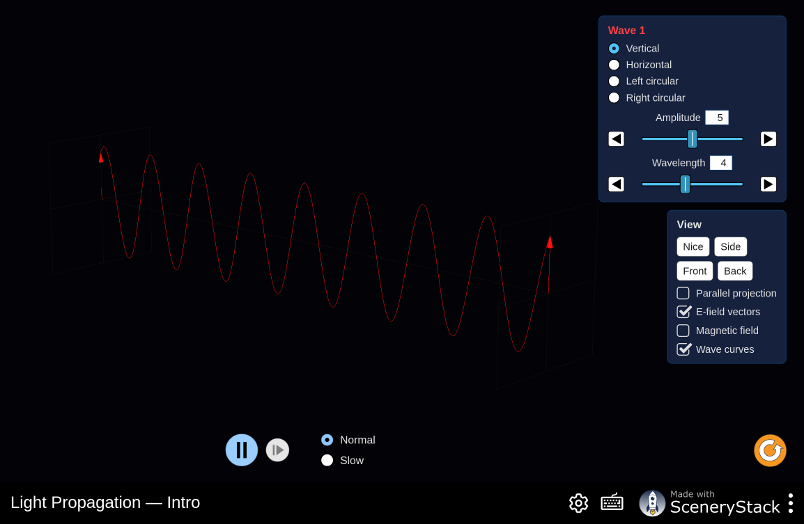
Figure 4.1:A monochromatic electromagnetic wave with its electric and magnetic fields drawn perpendicular to each other and to the direction of propagation. Later screens send the wave through polarizers and birefringent plates, where two components of one wave are given different optical paths — the same mechanism as the thin films of this chapter, applied to polarization rather than to geometry.
Interactive simulation: Light Propagation
Why Wave Effects Are So Hard to See
Before doing any interference calculation, it pays to understand why nobody notices these effects while walking around. The argument is a scaling argument, and it requires almost no algebra.
Suppose light of wavelength passes through an aperture of width and spreads by some angle . What can possibly depend on? The problem contains exactly two lengths, and , and is a pure number. A pure number cannot depend on a length, so it can only depend on the ratio of the two:
This is worth pausing on, because it says something strong. Shrink the wavelength and the aperture by the same factor and nothing changes — the whole pattern simply scales. It also means that experiments with water waves in a ripple tank, where wavelengths and apertures are both centimeters, are quantitatively informative about light, where both are tens of thousands of times smaller. What matters is never alone; it is .
The next chapter shows that for a slit the answer is , with no large numerical factor. Take that on trust for a moment and put in numbers. For green light, :
Through a pinhole, . Over a throw the beam spreads by about — comparable to the pinhole itself, and easily mistaken for the geometric shadow.
Through a gap the width of a human hair, , the spread is , giving about at . That is unmistakable, and it is why you can see diffraction by looking at a distant streetlight through a narrow gap between two fingers.
Through a doorway, , the spread is : about across a room. Utterly undetectable, which is why doorways cast sharp shadows.
So wave optics does not contradict the ray optics of an introductory course; it contains it. Ray optics is what wave optics becomes in the limit , and for everyday objects or smaller. This is an instance of the correspondence principle, an idea that will recur throughout this book: a more general theory must reproduce the older, more limited one in the regime where the older one was tested. Relativity reduces to Newtonian mechanics when (Chapter 2); quantum mechanics reduces to classical mechanics in the limit of large quantum numbers (Chapter 8); and wave optics reduces to ray optics when .
The practical lesson is simple: to see interference and diffraction, build apertures no more than a few hundred wavelengths across — that is, tenths of a millimeter or smaller. Young’s achievement was in large part an achievement of craftsmanship.
Huygens’s Principle
Huygens’s principle (1678) states that every point on a wavefront may be treated as a source of secondary spherical wavelets, spreading out at the wave’s speed; the wavefront at a later time is the envelope — the surface tangent to all of these wavelets.
This is a purely geometrical recipe, proposed nearly two centuries before Maxwell’s electromagnetic theory existed, and it is remarkably powerful. Applied to a plane wave in open space (Figure 4.2, panel a) it simply regenerates a plane wave, which is the least it must do. Applied at an interface it reproduces the laws of reflection and refraction. And applied at an aperture it makes a prediction that the ray picture cannot: the wavelets emitted near the edges have no neighbors to cancel their sideways spread, so the wave must bend into the geometric shadow. How much it bends depends, as the scaling argument above requires, on (panels b and c).
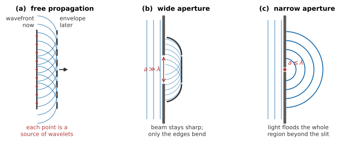
Figure 4.2:Huygens’s construction. (a) Each point of a wavefront emits a spherical wavelet; the envelope of the wavelets is the wavefront an instant later. (b) At an aperture much wider than a wavelength, the wavelets in the middle rebuild a flat wavefront and only the edges bend, so the beam looks like a ray. (c) When the aperture is comparable to a wavelength, a single wavelet survives and the transmitted wave spreads over the whole region beyond the slit. Original schematic generated with matplotlib; see scripts/figures/.
Two honest caveats. First, taken literally the construction also predicts a backward-traveling wave, which does not exist; Fresnel and later Kirchhoff repaired this by attaching an obliquity factor to each wavelet that suppresses backward emission, and by insisting that the wavelets be added with their phases rather than merely enveloped. That upgraded version — the Huygens–Fresnel principle — is the tool of Chapter 5. Second, Huygens’s principle by itself says nothing about intensity. To get intensities we need the superposition principle, which is where we turn next.
Superposition: Turning Path Difference into Phase Difference
The superposition principle states that when two or more waves overlap, the resulting disturbance at each point and each instant is the sum of the individual disturbances. For light this is a consequence of the linearity of Maxwell’s equations in vacuum and in ordinary transparent materials: fields add, and they add as vectors.
Consider two waves of the same frequency and the same amplitude arriving at some point . Suppose they left a common source in step with each other but then traveled different distances, and , to get to . Each accumulates phase at a rate of radians per wavelength traveled, so their phase difference at is
This one equation is the hinge of the whole chapter, and it is worth reading in both directions. A path difference of one whole wavelength corresponds to a phase difference of , which is no phase difference at all — the waves are back in step. A path difference of half a wavelength corresponds to a phase difference of , which puts crest against trough. In general:
Under constructive interference the fields add crest to crest, giving a resultant amplitude and — since — an intensity four times that of either wave alone. Under destructive interference the resultant amplitude is and the intensity vanishes. If the two amplitudes are unequal, the extremes are and ; complete darkness requires equal amplitudes, which is why interference fringes look best when the two slits are identical.
Three sources of phase difference will appear in this chapter, and it is worth naming them now so that they are not confused later:
Path difference in vacuum or air, — the double slit.
Optical path difference when part of the path lies in a medium, — thin films, and gas cells in an interferometer.
Phase shifts on reflection, an abrupt acquired at certain boundaries — thin films again.
Every interference problem in this chapter is solved by totaling these three contributions and asking whether the total is an even or an odd multiple of .
Worked Example: From Path Difference to Brightness
Two identical, in-step sources emit light of wavelength . At a particular point the waves have traveled distances differing by . Is that point bright or dark?
Count wavelengths in the path difference:
The path difference is two and a half wavelengths — a half-integer number — so , an odd multiple of . The point is dark.
Now suppose the whole region between the sources and that point is filled with water, , without moving anything. The geometric path difference is unchanged, but the wavelength in the water is , so the path difference is now wavelengths and the point is neither fully bright nor fully dark. Immersing an interference experiment in a medium genuinely changes the pattern; it does not merely rescale the brightness.
4.2Young’s Double Slit and Coherence
Young’s Double-Slit Experiment
Young’s arrangement is shown in Figure 4.3. Light from a source passes first through a single narrow slit, then through two narrow slits separated by a distance , and finally falls on a screen a distance away.
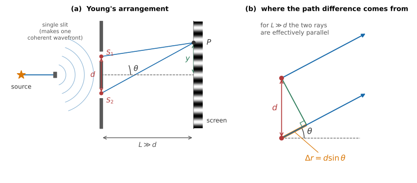
Figure 4.3:Young’s double-slit experiment. (a) The first slit produces a single wavefront that illuminates both of the second pair, so and act as coherent sources. (b) For the two rays reaching a distant point are effectively parallel, and the ray from travels an extra distance . Original schematic generated with matplotlib; see scripts/figures/.
The first slit is not decoration. Its job is to guarantee that a single wavefront reaches both of the following slits, so that whatever the source does — however erratically it flickers — it does the same thing at and at at the same moment. The two slits then behave as coherent sources with a fixed phase relationship. Without that first slit, different parts of an extended source illuminate the two slits independently, and the pattern washes out. (The coherence section below makes this precise; a modern laser has enough built-in coherence that the first slit can be omitted, which is why the classroom demonstration looks so much easier than Young’s original.)
The Path Difference
Consider a point on the screen, at angle from the central axis. Light reaching from has traveled farther than light from . Because in any practical apparatus — is tens of micrometers, is a meter or more — the two rays heading for are very nearly parallel, and the geometry collapses to the small right triangle of Figure 4.3(b): drop a perpendicular from onto the ray from , and the extra leg is
Combining this with the constructive and destructive conditions of the previous section gives the two-slit interference conditions:
The integer is the order of the fringe. The bright fringe sits on the axis, where the two paths are exactly equal; note that its position does not depend on , so in white light the central fringe is white while all the others are spread into little spectra.
Fringe Positions on the Screen
For small angles — again, the usual case — , where is measured on the screen from the central axis. The bright fringes then fall at
evenly spaced, with fringe spacing
Three features of this result deserve comment. First, measuring , , and determines — this was historically one of the first accurate measurements of the wavelength of visible light, and the first evidence that different colors correspond to different, specific wavelengths. Second, the fringes get farther apart as the slits get closer together: squeezing the apparatus stretches the pattern. This reciprocal relationship between a wave’s confinement and its spread is a hallmark of wave phenomena, and it returns as the uncertainty principle in Chapter 7. Third, the small-angle form is an approximation; when is only a few wavelengths the fringes are not evenly spaced and must be used directly.
The reciprocal relationship in is easy to state and easy to get backwards, so it is worth watching it happen. In Figure 4.4 the slit separation is a slider and the pattern responds live: closing the slits together spreads the fringes apart, and raising the frequency — shortening — packs them closer. The simulation runs the same geometry with water waves, sound, and light, which is a useful reminder that nothing in the derivation used any property of light beyond its being a wave with a wavelength.
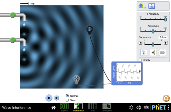
Figure 4.4:Young’s geometry with the slit separation, the slit width, and the wavelength under direct control. Switch between one slit and two: with one slit open the screen still shows structure, which is the diffraction of Chapter 5 intruding on the idealization used here, where the slits are treated as point sources.
Interactive simulation: Wave Interference
Finally, since can never exceed 1, the condition has solutions only for
so a double slit produces a finite number of orders — a point that becomes important for diffraction gratings in Chapter 5.
Worked Example: Wavelength from Fringe Spacing
Slits separated by are illuminated by a laser, and the resulting fringes on a screen away are found to be spaced apart. Find the laser wavelength.
Solving for :
consistent with a red helium–neon or diode laser. Note the sizes of the quantities involved: a wavelength has been measured with a millimeter ruler, because the apparatus magnifies the wavelength by the factor .
Worked Example: Fringe Angles, Positions, and Count
A double slit with is illuminated with the green line of a mercury lamp, , and the screen is away. (a) Find the angle to the third-order bright fringe. (b) Find the fringe spacing on the screen. (c) How many bright fringes appear on a screen wide, centered on the axis? (d) How many orders exist in principle?
(a) From with :
The angle is small, which retroactively justifies the small-angle work in (b).
(b)
(c) The screen extends from to , so the highest order that lands on it satisfies , giving . Orders through appear: seven bright fringes.
(d) In principle, . The far orders are useless in practice — they lie at large angles where the small-angle formula fails, and (as Chapter 5 shows) the finite width of real slits has long since dimmed them to nothing — but the counting matters for gratings.
Worked Example: The Same Experiment Under Water
The apparatus of the previous example is submerged in water, , source and screen included. What happens to the fringe spacing?
The frequency of the light does not change, but its wavelength does: . Nothing in the derivation of referred to vacuum, so the same formula holds with the local wavelength:
The pattern contracts by the factor . This is a genuinely useful check on understanding: it is the wavelength where the interference happens that sets the scale, and that is also why the thin-film formulas below carry a factor of .
Coherence
Young’s experiment works only because both slits are carved out of the same wavefront, so the light leaving them keeps a fixed phase relationship. Try the experiment with two separate light bulbs and you see nothing but a uniformly lit screen. The reason is not that light bulbs are dim; it is that they are incoherent.
An ordinary thermal source — a filament, a flame, a fluorescent tube — emits light as an enormous number of independent atomic events. Each excited atom radiates a short burst, a wave train lasting perhaps , and the next atom to radiate does so with no memory of the phase of the last. What emerges is therefore a chain of wave trains whose phase jumps randomly every few nanoseconds, as sketched in Figure 4.5.
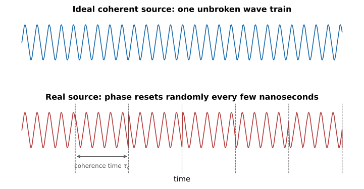
Figure 4.5:Coherence. An ideal source (top) maintains a predictable phase indefinitely. A real thermal source (bottom) emits short wave trains whose phase resets at random every coherence time ; any interference pattern formed by one train is replaced by a differently positioned pattern from the next, far faster than a detector can follow. Original schematic generated with matplotlib; see scripts/figures/.
Two independent sources therefore do produce an interference pattern — but a different one every few nanoseconds, in a random new position each time. Averaged over the nanoseconds to milliseconds that any real detector needs, the fringes wash out completely and the intensities simply add. The pattern is not weak; it is scrambled.
Temporal Coherence, Coherence Time, and Coherence Length
Two quantities measure how long a source stays predictable:
The coherence time : roughly the duration of one uninterrupted wave train, the time over which the phase remains predictable.
The coherence length : the corresponding path-length difference over which fringes survive. If the two arms of an interference experiment differ by much more than , the light recombining at the screen comes from two different, unrelated wave trains, and there is nothing stable to interfere.
Coherence length is set by the spectral purity of the source. A wave train of finite duration cannot be perfectly monochromatic — Fourier analysis gives it a spread of frequencies — and converting to wavelength gives the useful estimate
The representative values in Table 4.1 span an extraordinary range:
Table 4.1:Representative coherence lengths for common light sources
| Source | |||
|---|---|---|---|
| White light | (about two wavelengths) | ||
| Filtered sodium lamp | |||
| Helium–neon laser | |||
| Stabilized single-mode laser | hundreds of meters |
A closely related way to say the same thing: the number of fringes you can count before the pattern fades is roughly
White light gives you two or three fringes — which is exactly what Young saw, and exactly why the colored fringes of a soap bubble are confined to a film only a few wavelengths thick. A helium–neon laser gives several hundred thousand.
Spatial Coherence
Temporal coherence is about a single point in the beam staying predictable over time. Spatial coherence is about two different points across the beam having a fixed phase relationship at the same time, and it is what Young’s first slit provides. An extended source — the Sun’s disk, a broad filament — has poor spatial coherence, because light arriving at and light arriving at come from different, unrelated emitters. Passing the light through a pinhole first discards almost all of it but leaves what remains spatially coherent, since it all now originates from a region small enough to act as a single point.
A laser is coherent in both senses at once, which is why a laser pointer and a pair of razor-blade slits reproduce in seconds an experiment that took Young considerable ingenuity.
Worked Example: Will the Fringes Survive?
A Michelson interferometer (below) has arms differing in length by , so the two recombining beams differ in path by . Will fringes be visible with (a) a filtered sodium lamp, (b) a helium–neon laser?
(a) From Table 4.1, for the sodium lamp. The path difference of exceeds this by a factor of about 170, so the beams arriving together come from unrelated wave trains: no fringes.
(b) For the laser, , comfortably larger than the path difference: fringes are visible, though with reduced contrast since the path difference is a sizable fraction of .
This is not a contrived exercise. Michelson had to keep his arms equal to within a fraction of a millimeter precisely because his sodium light had a coherence length of well under a millimeter — a serious experimental constraint in 1887, and one that vanished with the invention of the laser.
4.3Intensity and Multiple Slits
Intensity: Adding Fields as Phasors
The conditions derived so far locate the bright and dark fringes but say nothing about the brightness in between. To get the full pattern we must add the two waves properly, and the most convenient bookkeeping for that is the phasor.
Because both waves have the same frequency, their relative phase does not change with time; only their common phase does. Represent each wave by a vector (a phasor) whose length is the wave’s amplitude and whose direction gives its phase. The whole diagram rotates rigidly at the optical frequency, so we may freeze it at any instant; adding the waves is then just adding the vectors, and the length of the resultant vector is the amplitude of the combined wave.
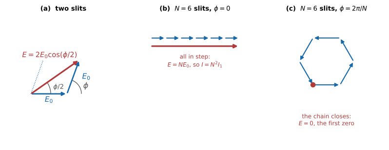
Figure 4.6:Phasor addition. (a) Two equal phasors separated by form an isosceles triangle whose base is the resultant, . (b) With slits and all the phasors line up, giving and hence . (c) When the chain closes on itself and the resultant vanishes — the first zero, at only of the way to the next principal maximum. Original schematic generated with matplotlib; see scripts/figures/.
Two Slits
For the double slit, two phasors of equal length are separated by the angle
They form an isosceles triangle (Figure 4.6(a)). The resultant bisects the angle between them, and dropping a perpendicular gives immediately
Squaring, and writing for the intensity one slit alone would produce,
The result is plotted in Figure 4.7. It reproduces everything derived earlier — whenever , and whenever — and now fills in the smooth variation between.
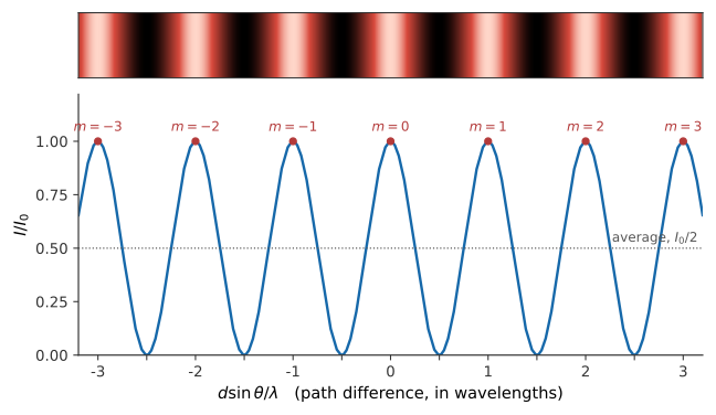
Figure 4.7:Two-slit intensity, , with the corresponding fringe pattern above. All the maxima have the same height and the fringes are evenly spaced — a signature of ideal, infinitesimally narrow slits. Real slits impose the envelope derived in Chapter 5. Generated with matplotlib; see scripts/figures/.
Where Does the Extra Light Come From?
The central maximum has intensity : four times what one slit would deliver, not twice. Students often find this alarming, and they should — until they check the energy budget.
The resolution is that averages to . Averaged across the pattern, the intensity is
which is exactly the two slits’ worth of light that entered. Interference does not create or destroy energy; it redistributes it, taking light from the dark fringes and piling it into the bright ones. The factor of four at the peaks is paid for by the zeros in between.
This is worth stating sharply, because it is the cleanest possible refutation of a classical particle picture of light: opening a second slit makes some places on the screen darker than they were with one slit open. No stream of independent corpuscles can do that.
Worked Example: Intensity Between the Fringes
For the mercury-lamp double slit above (, , ), at what distance from the center of the pattern does the intensity fall to half its maximum?
Set :
So the half-intensity point occurs at a quarter-wavelength path difference — one quarter of the way from a bright fringe to the next dark one. In small-angle terms :
The full width at half maximum of each fringe is therefore , exactly half the fringe spacing in this small-angle approximation. Two-slit fringes are broad and sinusoidal — which, as the next section shows, is precisely what more slits fix.
Three Slits, and Then 
Add a third identical slit, equally spaced. What changes?
The principal maxima do not move. At , every slit is in step with every other, so all three phasors point the same way, the resultant is , and the intensity is . Adding slits at the same spacing can never shift these directions; it just adds more phasors to an already aligned stack.
What changes is where the first zero falls. With two slits, the resultant vanishes when the second phasor is antiparallel to the first: . With three slits, the three phasors close into an equilateral triangle — and hence sum to zero — as soon as , well before reaches . The maximum has become narrower. With slits, the chain closes into a regular -gon at (Figure 4.6(c)), so the first zero sits only of the way to the next principal maximum.
Summing the general chain is a geometric series. Writing each successive phasor as the previous one multiplied by , the total field is , whose magnitude works out to . Squaring gives the -slit intensity pattern
where is the intensity from a single slit. Setting recovers the two-slit result, since .
Summing the -slit phasor chain
The total field at angle is the sum of equal-amplitude phasors, each rotated by from the last:
This is a finite geometric series with common ratio , so
To get the magnitude, factor a half-angle phase out of both numerator and denominator: for any angle , . Applying this with in the numerator and in the denominator,
The prefactor has magnitude 1 — it is only an overall phase, reflecting the arbitrary choice of the first slit as the phase origin — so the amplitude is
exactly the result quoted in the main text. Squaring gives the -slit intensity formula, and setting recovers the two-slit result via the identity .
Figure 4.8 collects the consequences:
Principal maxima occur wherever is a multiple of , that is — the same directions as for two slits, for any . Their height is .
Zeros occur at for every integer that is not a multiple of . There are zeros between consecutive principal maxima, and hence much weaker secondary maxima squeezed between them.
Width. Since the first zero is at , the angular half-width of a principal maximum scales as : doubling the number of illuminated slits halves the width of every line.
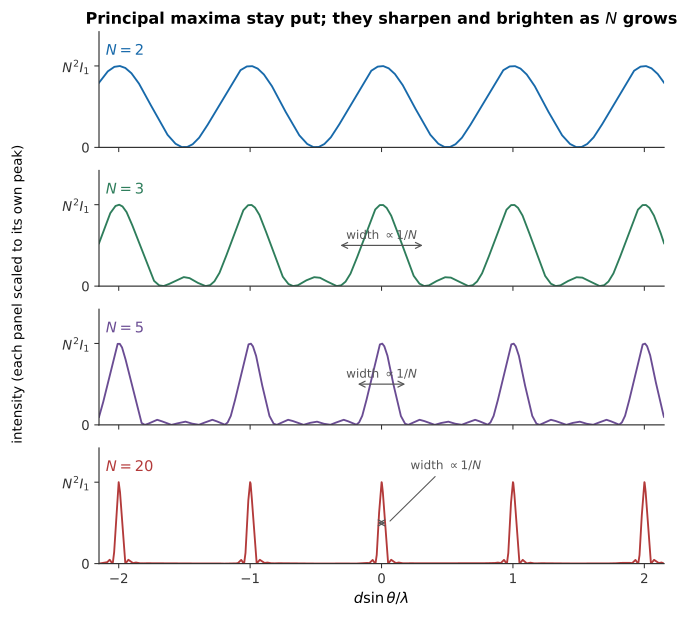
Figure 4.8:Interference from equally spaced ideal slits. The principal maxima stay at regardless of , but they grow taller (peak ) and narrower (width ), and weak secondary maxima appear between them. Each panel is scaled to its own peak. Generated with matplotlib; see scripts/figures/.
The two scalings work together. The peak height grows as while the width shrinks as , so the energy in each principal maximum grows only as — as it must, since slits admit times as much light. What you gain by adding slits is not more light in total but light concentrated into sharper and sharper spikes at precisely determined angles. Since those angles depend on , a device with very many slits becomes an extremely precise wavelength meter. That device is the diffraction grating, and it is taken up — together with the complication that real slits have finite width — in Chapter 5.
Worked Example: Locating the Zeros of a Five-Slit Pattern
Five slits with are illuminated at . Find the directions of the principal maxima, and of the zeros lying between the central maximum and the first-order maximum.
Principal maxima: , giving at , plus exactly at (grazing, and not observable).
Zeros: means , so
for (the value is excluded — it is the first-order principal maximum). The four zeros lie at , and between them sit secondary maxima. Note that the first zero is at , one fifth of the way to the first principal maximum at 0.250. For comparison, the first zero of the two-slit pattern is halfway to that maximum, so this five-slit central peak is 2.5 times narrower than the corresponding two-slit peak.
4.4Thin Films and Interferometers
Thin-Film Interference
The most familiar interference in everyday life needs no slits at all. The colors swirling on a soap bubble, the rainbow sheen of oil on a wet road, and the faint purple cast of a coated camera lens are all produced by light reflecting from the two surfaces of a very thin transparent layer.
Figure 4.9 shows the situation. Light striking a film of thickness and refractive index partially reflects at the front surface (ray 1) and partially enters the film, reflects from the back surface, and re-emerges (ray 2). The two emerging beams are parallel, and the eye or a lens brings them together to interfere.
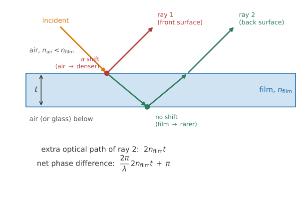
Figure 4.9:Thin-film interference. Ray 1 reflects from the front surface, where the index increases, and picks up a phase shift. Ray 2 makes a round trip inside the film, acquiring an extra optical path , and reflects from the back surface, where the index decreases, with no shift. The net phase difference is the sum of the two effects. Original schematic generated with matplotlib; see scripts/figures/.
The Two Contributions
Optical path. At near-normal incidence, ray 2 travels an extra geometric distance , all of it inside the film. By the optical-path rule, this corresponds to a phase difference of
with the vacuum wavelength. The factor is not optional: the film packs more wavelengths into the same thickness.
Phase shift on reflection. Reflection at a boundary where the refractive index increases (light in a lower-index medium striking a higher-index one) flips the sign of the reflected field — an extra phase shift of exactly . Reflection at a boundary where the index decreases produces no shift. The mechanical analog is a wave on a string: a pulse reflecting from a fixed end (a heavy string beyond, the “denser” case) comes back inverted, while a pulse reflecting from a free end (a light string beyond) comes back upright. “Higher refractive index” plays the role of “heavier string”.
That analog is worth more than a sentence, because the sign is the one thing students reliably get wrong and it is not something to be memorized. Figure 4.10 launches a pulse down a chain of masses and springs terminated either rigidly or freely, and the inversion is not scripted into the simulation: it falls out of the boundary condition, exactly as the shift falls out of matching the electric field across an optical interface. A fixed end cannot move, so the reflected pulse must arrive with the opposite sign to cancel the incident one there; a free end has nothing to push against, and the pulse returns upright.
Figure 4.10:A pulse reflecting from a rigid termination and from a free one, side by side on the same clock. The rigid end inverts the pulse and the free end does not — the mechanical statement of the 0-or- rule used throughout this section.
Interactive simulation: Standing Waves
Assembling the Conditions
Because the reflection shifts are either 0 or , the two reflections in Figure 4.9 can only produce a net relative shift of 0 or . This gives a reliable three-step recipe:
Check the front reflection. Does the index increase going into the film? If so, that ray gets .
Check the back reflection. Does the index increase going out of the film into whatever lies beyond? If so, that ray gets .
If exactly one of the two picked up , the net reflection shift is ; if both did or neither did, it is 0.
Case A — net shift of (exactly one reflection flips). This covers a soap film in air, an oil slick on water, and an air gap trapped between two glass plates. Bright reflection needs the path contribution to supply the missing half wavelength:
Case B — net shift of 0 (both flip, or neither does). This covers any film whose index lies between those of the media on either side — an antireflection coating on glass, or an oil film on a denser substrate. The conditions are exactly reversed:
Getting the case wrong swaps bright for dark everywhere, so it is worth the ten seconds it takes to check.
Why Soap Films Are Colored — and Why They Go Black
Since the conditions involve , a film illuminated with white light reflects some wavelengths strongly and suppresses others, and the favored wavelength shifts as the thickness changes. Figure 4.11 shows the reflected intensity of red, green, and blue light as a function of the thickness of a soap film in air.
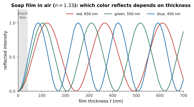
Figure 4.11:Reflected intensity from a soap film in air () versus film thickness, for three visible wavelengths. Different colors peak at different thicknesses, which is why a draining soap film shows moving bands of color. As all three curves go to zero: the film turns black just before it bursts. Generated with matplotlib; see scripts/figures/.
Two features of the figure are worth dwelling on. First, the three curves peak at different thicknesses, so a soap film whose thickness varies from place to place — as it always does, since gravity drains it — shows bands of color that drift downward as the film thins. Second, and more striking: as all the curves go to zero. A film very much thinner than contributes almost no path difference, so the two reflections are left with only the shift and cancel for every visible wavelength at once. The film goes black — a genuinely counterintuitive prediction, and one you can verify by watching a soap film held vertically in a wire loop: a black band appears at the top, spreads downward, and moments later the film bursts. Newton described this effect in the 1670s, without being able to explain it.
Worked Example: The Color of a Soap Film
A soap film () in air is thick. Which visible wavelength does it reflect most strongly, viewed at normal incidence?
This is Case A (air–film–air, so only the front reflection flips), and constructive reflection requires . Solving for :
For : — green. For : , deep in the ultraviolet and invisible. So this film looks green, and only the order matters. That is characteristic of thin films: they are thin enough that only the lowest one or two orders land in the visible, which is why their colors are broad and pastel rather than a sequence of sharp spectral lines.
Worked Example: An Antireflection Coating
A camera lens () is coated with magnesium fluoride () to minimize reflection at , the middle of the visible spectrum where the eye is most sensitive. Light is incident from air. Find the minimum coating thickness.
Apply the recipe. Front reflection: air (1.00) into (1.38) — index increases, so . Back reflection: (1.38) into glass (1.52) — index increases again, so . Both flip: this is Case B, net shift 0, and destructive reflection requires the odd-quarter-wave condition
The thinnest coating uses :
the standard “quarter-wave” coating. Two remarks. First, the cancellation is not perfect even at , because the two reflected beams have slightly different amplitudes; complete cancellation would require , and at 1.38 is simply the closest durable material available. Second, the condition is wavelength-specific: at and the same coating still suppresses reflection, but only partially. The residual reflection is therefore richer in blue and red than in green, which is exactly the faint purple sheen you see on a coated lens.
Wedges and Newton’s Rings
A film need not have uniform thickness. Press two flat glass plates together and separate one edge with a thin spacer — a hair, a wire, a sheet of paper — and the air gap between them forms a wedge whose thickness grows linearly along the plates. This is Case A: at the glass-to-air surface the index decreases, so there is no shift, while at the air-to-glass surface below it increases, so that reflection flips. Exactly one flip, net shift , and with for air the dark fringes fall where — including at , so the line of contact is dark. That dark contact line is a useful check that you have assigned the case correctly.
If the wedge has thickness at a distance from the contact line, then at position , and successive dark fringes are separated by
Counting the fringes over the whole length gives , so the wedge is a way of measuring a very small thickness by counting a large number.
Replace the top plate with a slightly convex lens resting on the flat and the fringes become concentric circles: Newton’s rings. For a lens of radius of curvature , geometry gives the gap at radius as , so the dark rings fall at
with a dark spot at the center. The rings crowd together as grows, since . Newton’s rings remain a standard optical-shop test: any departure of the ring pattern from perfect circles reveals a departure of the surface from a perfect sphere, at a sensitivity of a fraction of a wavelength.
Worked Example: Measuring a Wire with an Air Wedge
Two flat glass plates long are in contact at one end and separated at the other by a thin wire. Illuminated from above with sodium light (), the plates show 170 dark fringes between the contact line and the wire. Find the wire’s diameter.
The wire’s diameter is the wedge thickness at the far end. Dark fringes occur wherever , so the fringe count from to is :
The plate length never entered — it only sets the fringe spacing, , which is what makes the fringes countable by eye. A wire has been measured to within a fraction of a micrometer using nothing but two pieces of glass, a sodium lamp, and patience.
The Michelson Interferometer
The Michelson interferometer (Figure 4.12) is Young’s two-path experiment rebuilt with mirrors, and it is the most consequential single instrument in this book.
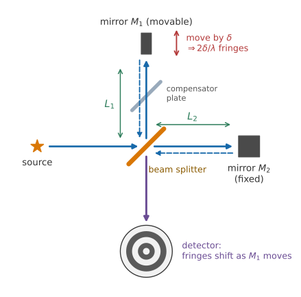
Figure 4.12:The Michelson interferometer. A beam splitter divides the incoming light into two perpendicular arms; each returns from a mirror and the two recombine at the splitter. Moving one mirror by changes that arm’s round trip by and sweeps fringes past the detector. The compensator plate equalizes the amount of glass traversed by the two beams. Original schematic generated with matplotlib; see scripts/figures/.
A beam splitter — a half-silvered mirror — divides an incoming beam into two perpendicular paths of lengths and . Each path ends at a mirror that sends the light back, and the beam splitter recombines the two returning beams and sends them to a detector. The round-trip path difference is , so the recombined beams interfere according to
Now translate one mirror through a distance . That arm’s round trip changes by , and the fringe pattern shifts by
One full fringe passes the detector for every half wavelength of mirror motion. Since for visible light, and fringe positions can be interpolated to a small fraction of a fringe, the instrument measures displacements of a few nanometers. That is the whole reason for its importance: it converts a length comparison into a fringe count, and light’s wavelength is a very fine ruler.
The small tilted plate in Figure 4.12 is the compensator. Without it, the beam going to passes through the glass of the beam splitter three times while the beam going to passes through it once — a large and, worse, wavelength-dependent optical path difference. The compensator is an identical piece of uncoated glass placed in the other arm so that both beams traverse the same thickness. It is unnecessary with a laser but essential with white light.
Both arms, and the fringes they produce, can be manipulated directly in Figure 4.13. Translating one mirror sweeps the fringe count given by Equation (4.47); shortening the coherence length washes the fringes out, which is the coherence-length constraint of the earlier section made visible.
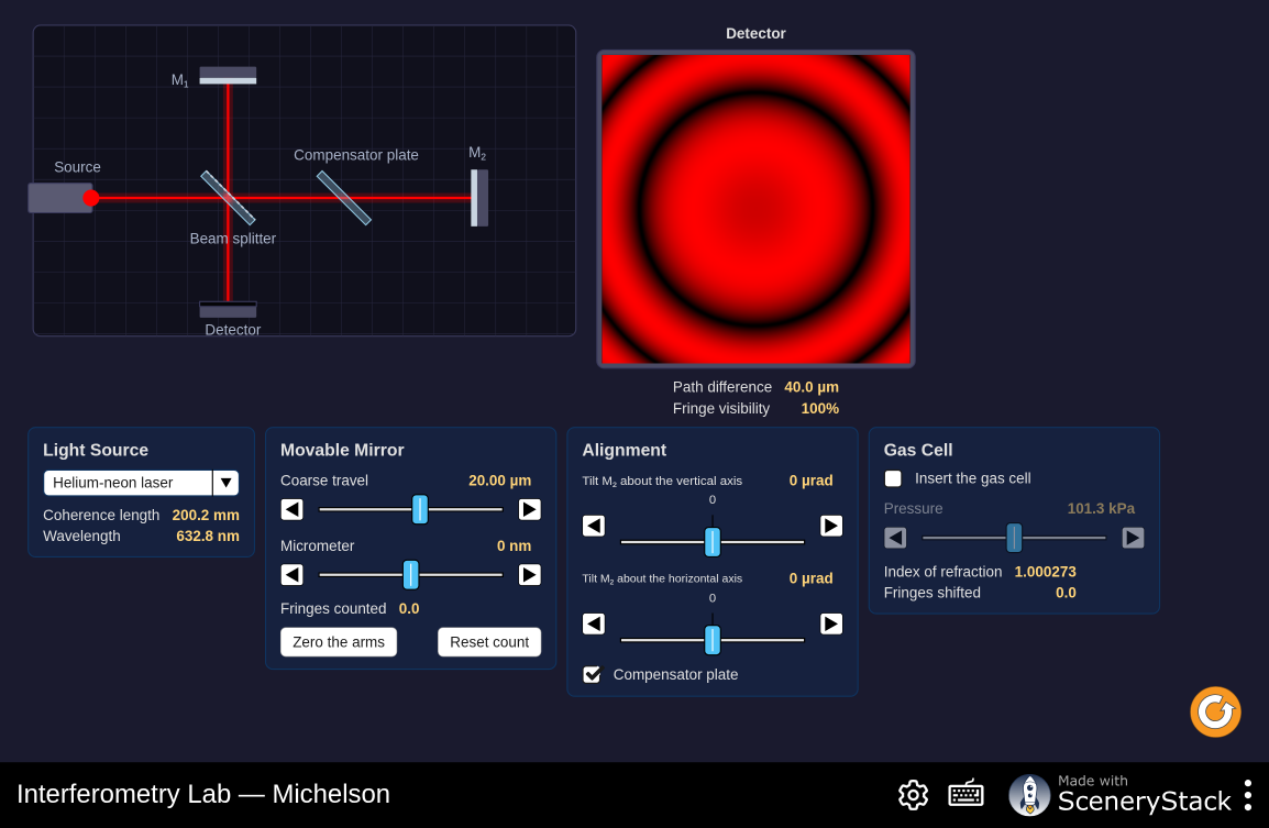
Figure 4.13:A physical-optics model of the Michelson interferometer, together with the Mach–Zehnder and Fabry–Pérot geometries. Move a mirror and count fringes; change the source’s coherence length and watch the visibility collapse.
Interactive simulation: Interferometry Lab
Worked Example: Counting Fringes
In a Michelson interferometer illuminated with sodium light, , one mirror is slowly translated and 1200 fringes are counted passing a reference mark. How far did the mirror move?
Note the leverage: a third of a millimeter of motion, resolved into 1200 countable events.
Worked Example: The Refractive Index of Air
A transparent cell of length is placed in one arm and slowly evacuated. As the air is pumped out, 49.7 fringes are counted. Find the refractive index of air at .
The light crosses the cell twice, so removing air of index changes the optical path by , and the fringe count is
so — the accepted value for dry air at standard conditions. The interferometer has measured a refractive index that differs from unity in the fourth decimal place, from a fringe count that a student can do by eye.
What Interferometers Are For
The Michelson–Morley experiment. As described in Chapter 1, rotating the apparatus should have exchanged the roles of the arm parallel to Earth’s motion through the ether and the arm perpendicular to it, shifting the fringes by about 0.4 fringe against a sensitivity of 0.01 fringe. No shift was ever seen, at any orientation or any time of year. The fringe-counting relation in Equation (4.47) is exactly what converted a null optical measurement into a decisive statement about the structure of spacetime.
Fourier-transform spectroscopy. Record the detector signal as a function of mirror position and you have the autocorrelation of the light; its Fourier transform is the spectrum. Nearly every infrared spectrometer in a modern chemistry laboratory is a Michelson interferometer operated this way.
Metrology. Surface flatness, machine-tool calibration, and — until the 1983 redefinition of the meter in terms of — the international length standard itself.
Gravitational-wave detection. LIGO and Virgo are Michelson interferometers with arms, folded optically to an effective length of hundreds of kilometers, measuring mirror displacements of order — about one ten-thousandth of a proton’s diameter. The first detection, in September 2015, came from two merging black holes 1.3 billion light-years away. The instrument that failed to find the ether became the instrument that found the ripples in spacetime that replaced it.
Looking Ahead: Interference One Photon at a Time
Everything in this chapter treats light as a classical wave, and the treatment works. It is worth flagging now, though, that the story does not end here.
Turn the source in Young’s experiment down. Not a little — down until the light is so faint that, on average, only one quantum of light is inside the apparatus at any moment. A helium–neon laser emits about photons per second; light crosses a meter-long apparatus in about . A rate below roughly 108 photons per second keeps the mean number of photons in the apparatus below about 0.3; individual emission intervals are still random, but simultaneous photons are then uncommon. G. I. Taylor performed the experiment in 1909 using an attenuated gas flame and a three-month exposure, and it has been repeated countless times since with single-photon sources and imaging detectors.
The result is that the screen records individual, localized hits — dots, one at a time, apparently at random. But as the dots accumulate over hours, they build up precisely the fringe pattern derived in this chapter. The probability amplitude associated with each photon interferes between the two paths; there is no second photon for it to interfere with. That fact cannot be accommodated by any picture in which the photon simply goes through one slit or the other, and it is the central puzzle that Chapters 6 and 7 take up.
For now, the wave description stands on its own, and the next chapter completes it.
4.5Summary
Light is an electromagnetic wave. Detectors measure the time-averaged intensity, , so amplitudes superpose and the intensity is the square of the sum — never the sum of the intensities. In a medium of index , the wavelength shrinks to , and what governs interference is the optical path length .
Wave effects hide behind a small number. The only dimensionless quantity available is , and for everyday apertures it is . Ray optics is wave optics in the limit — an instance of the correspondence principle.
Huygens’s principle treats every point of a wavefront as a source of secondary wavelets whose envelope is the later wavefront; it predicts that waves spread after an aperture, by an amount governed by .
Path difference becomes phase difference through . Constructive interference requires , destructive requires .
Young’s double slit gives bright fringes at and dark fringes at ; for and small angles, the fringes are evenly spaced with . Only orders with exist.
Coherence is required for a stable pattern. Real sources emit short wave trains with randomly resetting phase; the coherence time and coherence length set the largest usable path difference, and estimates the number of visible fringes. Spatial coherence — supplied by Young’s first slit, or built into a laser — is what lets two slits act as one source.
Phasor addition gives the two-slit intensity with . The factor of four is offset by the zeros: the pattern redistributes energy, averaging back to .
equally spaced slits give . Principal maxima stay at , rise as , and narrow as , with weak secondary maxima between them — the basis of the diffraction grating (Chapter 5).
Thin films interfere via the extra optical path plus any shift from reflection at a boundary where the index increases. Count the shifts first: one flip gives constructive reflection at ; zero or two flips reverse the conditions. This explains soap-film colors, the black film, quarter-wave antireflection coatings, wedge fringes, and Newton’s rings ().
The Michelson interferometer converts a mirror displacement into a fringe count , giving nanometer sensitivity. It produced the null result of Chapter 1, and, scaled to kilometers, the first detection of gravitational waves.
4.6Conceptual Questions
Two flashlights are aimed at the same spot on a wall. Explain, in terms of coherence time, why no interference fringes appear, even though two light waves are certainly overlapping there.
In Young’s experiment, what happens to the fringe spacing if (a) the slit separation is doubled, (b) the screen distance is doubled, (c) the light is changed from red to blue, (d) one slit is covered? Answer each in one sentence.
The central maximum in a double-slit pattern has four times the intensity that one slit alone would produce. Explain why this does not violate conservation of energy, and state where the extra energy comes from.
Explain why the fringe is white when a double slit is illuminated with white light, while every other fringe is colored.
A soap film held vertically in a wire loop develops a black band at the top just before it bursts. Explain why the film appears black there rather than showing some color, and why the band appears at the top.
A camera lens with an antireflection coating still shows a faint purple reflection. Explain why the coating cannot eliminate reflection at all visible wavelengths at once.
Two glass plates in contact at one edge form an air wedge. Is the fringe at the line of contact bright or dark? Justify your answer by counting phase shifts on reflection, and explain what you would conclude if you observed the opposite.
Explain why a Michelson interferometer with arms differing by several centimeters shows fringes with a laser but not with a sodium lamp, even though the sodium lamp is far from white.
4.7Problems
Solution to Exercise 4.1 #
Solution to Exercise 4.2 #
For small angles, adjacent bright fringes are separated by , so
Therefore, the light has wavelength about , which is yellow light.
Solution to Exercise 4.3 #
Solution to Exercise 4.4 #
For in-step sources, a bright point requires and a dark point requires . Hence
Also first occurs at , so and . Therefore, the smallest nonzero path differences are (bright), (dark), and (half maximum).
Solution to Exercise 4.5 #
Immersion changes the wavelength to while and remain fixed. Thus
Therefore, the new fringe spacing is ; it depends only on the optical path difference between the two complete paths, so moving the liquid within an apparatus that is wholly immersed cannot change it.
Solution to Exercise 4.6 #
The coherence length is approximately . For the laser,
and the number of wavelengths, hence the approximate number of visible fringes, is . For white light,
Therefore, the laser can show about fringes over a path mismatch, whereas white light shows only a few fringes because its wavelengths lose phase agreement almost immediately.
Solution to Exercise 4.7 #
At half maximum, , so the two nearest values are and therefore . Since , the two half-maximum points obey
Their separation is . Adjacent bright fringes differ by , so the FWHM is in this coordinate, exactly one-half of the fringe spacing. In the small-angle approximation, , so the same ratio holds on the screen: the FWHM is one-half the bright-fringe spacing, independently of , , and . At larger angles the exact screen-coordinate widths and spacings are not uniform.
Solution to Exercise 4.8 #
At , all phases agree and the -slit formula gives . Consequently,
so doubling the slit number from 2 to 4 raises the peak height by , confirming . The principal-maximum angular width is proportional to , so peak height times width scales as . Therefore, coherent addition makes a peak taller as , but its narrowing ensures that the total transmitted light is proportional only to the number of slits.
Solution to Exercise 4.9 #
Principal maxima obey , hence
The allowed orders are , with , the last pair falling exactly at (grazing, and not observable). Zeros satisfy where between adjacent principal maxima. Between and , , giving . There are secondary maxima between those five zeros, as shown in Figure 4.14.
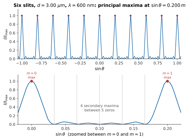
Figure 4.14:Six-slit pattern for , . Top: principal maxima at . Bottom: zoom between and , showing the five zeros and four secondary maxima predicted above.
Therefore, the stated principal directions, five intervening zeros, and four secondary maxima describe the six-slit pattern.
Solution to Exercise 4.10 #
The air-to-film reflection is from lower to higher index and gains a phase shift; the film-to-air reflection is from higher to lower index and gains none. This is the one-phase-reversal case. Bright reflection therefore requires :
For , and . Dark reflection requires , and its smallest nonzero thickness is
Therefore, the first two bright thicknesses are and , and the first nonzero dark thickness is .
Solution to Exercise 4.11 #
For oil on water, the air--oil reflection reverses phase but the oil--water reflection does not, so this is the one-reversal case (Case A). Its first bright thickness is
For oil on material, both reflections reverse phase, so this is Case B. Bright reflection then requires , whose first nonzero solution is
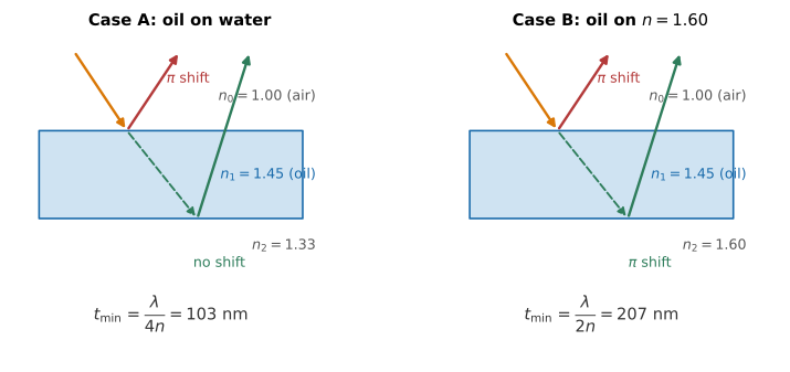
Figure 4.15:Case A (oil on water) has one phase reversal, so the first bright thickness is a quarter-wave; Case B (oil on the denser substrate) has two reversals that cancel, so the first bright thickness is a half-wave — twice as large.
Therefore, oil on water is Case A and reflects strongly first at , while oil on is Case B and first reflects strongly at ; the two phase reversals shift the condition by half an order.
Solution to Exercise 4.12 #
Both air--coating and coating--glass reflections reverse phase, so destructive reflection requires a quarter-wave thickness:
For this thickness, . Thus it is at and at , rather than the design value 0.500. Therefore, a coating minimizes reflection, but it is imperfect at blue and red wavelengths; the unequal residual reflection can look purple.
Solution to Exercise 4.13 #
For reflected Newton rings with one phase reversal, dark rings satisfy . Hence
At the center , the propagation phase difference is zero while one reflected ray has a shift, so the center is dark. Since , decreases as increases, as seen in Figure 4.16.
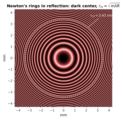
Figure 4.16:The reflected pattern: dark at the center from the single phase reversal, with so the rings crowd together as grows. The dashed circle marks .
Therefore, the tenth dark ring has radius , the center is dark because of the single phase reversal, and rings crowd outward.
Solution to Exercise 4.14 #
Solution to Exercise 4.15 #
A mirror displacement changes the round-trip path by , so
Therefore, about 733 fringes pass the reference mark.
Solution to Exercise 4.16 #
Solution to Exercise 4.17 #
Inside a film the wavelength is , so a round-trip geometric distance contains wavelengths; this is why the optical path is . Omitting for a soap film would predict a phase corresponding to rather than , an error of in optical path, or of a visible-light wavelength near . More concretely, the correct lowest-order bright wavelength is , whereas dropping would predict , shifting the prediction from green to violet. Therefore, dropping produces a substantial phase and color error, not a small correction.
Solution to Exercise 4.18 #
The path difference is , so the fringe shift is
A rotation exchanges the arms and doubles the change, giving about 0.37 fringe, consistent with the historical prediction. Therefore, the expected shift was roughly 0.4 fringe, about 40 times the 0.01-fringe sensitivity.
Solution to Exercise 4.19 #
The round-trip phase count is
Therefore, a LIGO-scale displacement is only about of a fringe in one pass, so real detectors must amplify the effective path with optical cavities and reduce statistical noise by averaging very large photon counts.
Solution to Exercise 4.20 #
Coincident bright fringes require . For and ,
The smallest positive integers are and . The common position is
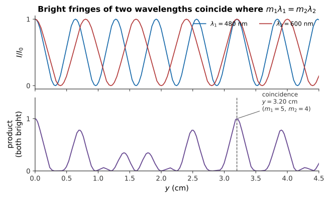
Figure 4.17:The two fringe patterns drift in and out of step; their product (bottom) peaks wherever both are bright at once, first at where and .
Therefore, the first noncentral coincidence is from the center.