9. Steam Power Cycles - Engineering Thermodynamics

9. Steam Power Cycles¶

Steam Power Cycles

The Understated Charm of Thermal Power Plant Water Circuits

Introduction¶

Now that we have acquired solid theoretical concepts, we can take a closer look at the thermodynamic cycles used in industry. This chapter 9 (steam

power cycles) aims to answer two questions:

• Why and how are steam engines used today?

• Why are we moving away from ideal cycles and how do we quantify these compromises?

9.1 Why Use a Steam Engine?¶

« Attempts have been made, on various occasions, to make heat act upon atmospheric air in order to give birth to motive power. This gas presents, in comparison to water vapor, some advantages and some disadvantages which we shall now examine. 1°. It offers, relative to water vapor, a notable advantage in that, possessing at equal volume a far lesser capacity for heat, it would cool to a greater degree by a similar expansion in volume. […] Now, we have seen how important it is to induce, by changes in volume, the greatest possible variations in temperature. 2°. Water vapor can only be formed through the intermediary of a boiler, whereas atmospheric air could be heated directly by combustion executed within it. One would thus avoid a considerable loss, not only in the quantity of heat, but also in its thermometric degree. »

Sadi Carnot, 1824 [4]

The use of water as a working fluid in a machine undeniably has many disadvantages. In particular, unlike internal combustion engines:

• It is necessary to either recycle the water in the machine (and therefore cool it), or find a continuous source of pure water to operate it;

• There is an inevitable loss of some of the heat supplied to the machine, above the boiler.

Why, then, be interested in the operation of steam engines? The answer is that many sources of heat do not allow heat to be brought directly inside the working fluid. At the end of combustion, coal, wood, household or agricultural waste, for example, leave significant residues that cannot be circulated in a turbine. As for nuclear reactions, they cannot be carried out directly within the air. The exploitation of these sources, which accounts for a significant share of the world’s sources of mechanical or electrical energy, therefore requires extracting heat from outside the engine.

Liquids have an excellent volumetric thermal capacity compared to that of air (as the student will find using both chapter 4 and 5, that of liquid water is approximately a thousand times higher): they are compact mediums for extracting heat from an external source. Among them, water is the most abundant and certainly the least difficult to handle. Thus, almost every time the heat input cannot be made within air, water is chosen as the engine’s working fluid.

The sources of heat used by steam engines make their use in transportation difficult, so they are most often used in static installations to generate electricity: a configuration that allows economies of scale in energy storage and transport. All these factors justify the development of steam power plants with several gigawatts of electrical power $(1 GW = 10^{9}W)$ , making them the most powerful thermal engines in the world.

9.2 Engine Evaluation Criteria¶

Several parameters are taken into account in the evaluation of the performance and value of steam engines.

9.2.1 Thermal efficiency and overall efficiency¶

The parameter that we have learned to quantify so far is of course the thermal efficiency of the engine $\eta _{\mathrm{engine}}\equiv \left|\frac{\dot{W}_{\mathrm{net}}}{\dot{Q}_{\mathrm{in}}}\right|$ (6/4) that we always strive to maximize towards its theoretical maximum, $\eta _{\mathrm{Carnot\ engine}}= 1- \frac{T_{\min.}}{T_{\max.}}$ (7/6).

However, it is important not to forget that the conversion of heat into work is just one of the many operations involved in electricity production:

• Fuel preparation (refinement and heating of oil, coal pulverization, separation of oil sands) itself may require energy, which we can evaluate with an efficiency $\eta _{\mathrm{preparation}}$ ;

• In the boiler, the energy transfer from the heat source to the water can be incomplete (with some heat potentially being rejected with the exhaust gases), which we can evaluate with an efficiency $\eta _{\mathrm{boiler}}$ ;

• The transmission of mechanical energy from the turbine to the generator, possibly using a gearbox, incurs friction losses that we evaluate with an efficiency $\eta _{\mathrm{transmission}}$ ;

• The transformation of shaft power into electrical power also involves losses resulting in the production of heat, which we evaluate with an efficiency $\eta _{\mathrm{generator}}$ .

Thus, the overall efficiency $\eta _{\mathrm{overall}}$ of electricity production at the output of the power plant, which compares the electrical energy produced to the actual heat spent to generate it (in other words, its energy cost), is the product of all these efficiencies:

\eta _{\mathrm{overall}}\equiv \eta _{\mathrm{preparation}}\eta _{\mathrm{boiler}}\eta _{\mathrm{engine}}\eta _{\mathrm{transmission}}\eta _{\mathrm{generator}}

(9/1)

Engineers are expected to work on increasing the overall efficiency rather than just $\eta _{\mathrm{engine}}$ . It may be acceptable to intentionally reduce thermal efficiency if it allows, for example, an increase in $\eta _{\mathrm{boiler}}$ (with better heat extraction from the flue gases) or $\eta _{\mathrm{generator}}$ (with an increase in turbine speed).

9.2.2 Power and specific consumption¶

The efficiency of an engine is not the only parameter we consider in the economic evaluation of its use: the costs associated with its maintenance or supervision of its operation, and of course the acquisition costs, are also crucial. These expenses can only be calculated if we delve into technological details that go beyond the scope of this book.

Despite this, we can already crudely assess the size and acquisition cost of an engine by calculating its specific net power $w_{\mathrm{net}}$ . In order to be compact, it is indeed desirable for an engine to generate a large net power for a given mass flow rate: it may even be desirable to compromise thermal efficiency for this purpose.

In industry, it is more common to measure the inverse parameter, which we call specific steam consumption. This consumption indicates the steam flow rate required to supply one watt of useful power. We denote it as ssc:

\mathrm{ssc} \equiv \frac{1}{|w_{\mathrm{net}}|}

(9/2)

where ssc is the specific consumption $(kg J^{-1})$ , and $w_{\mathrm{net}}$ is the specific power delivered by the machine $(J kg^{-1})$ .

The unit of specific consumption is $kg J^{-1}$ (representing $kg s^{-1}$ of water per $W$ of power), but the common practice in industry is to measure it in $kg/(kW h)$ (kilograms per kilowatt-hour).

9.2.3 Environmental impact¶

The production of heat in thermodynamic engines is at the heart of the major ecological challenges of our century. A comprehensive study goes beyond the scope of this book, so we will only note that the environmental impact can be divided into three main categories:

• Pollution by emission of harmful particles from combustion, particularly concerning the combustion of solids (especially coal as well as household and agricultural waste). With a filtering system, these emissions can generally be reduced to a very low level;

• Emission of greenhouse gases, especially CO $_{2}$ , an inevitable product of the combustion of hydrocarbons which is now known to be a major contributor to global climate change. These emissions concern all heat sources based on combustion;

• Emission of radioactive waste, which concerns nuclear heat sources. These wastes are in small quantities but remain harmful for time periods counted in millennia.

Thus, apart from a few rarely-available heat sources (geothermal or solar concentration), thermodynamic engines are always powered by sources with major disadvantages. However, they are still the only ones that provide us with abundant energy in mechanical and electrical form, and this abundance is tightly coupled with the economic and societal progress our civilization made in the last two centuries. It is up to responsible engineers and citizens to judiciously assess their flaws and qualities.

9.3 Components of Steam Power Plants¶

Before studying the construction of steam thermodynamic cycles, we briefly review the operation mode of the most common components of power plants.

9.3.1 Calculation of component powers¶

All steam systems used today operate with a continuous flow rate. Also, in these machines, the changes in the steam’s kinetic and potential energy are small compared to heat and work transfers. We will therefore exclusively use the concepts covered in chapter 3 (open systems) and we will be able to relate the powers and the thermodynamic state of the steam using the simple equation:

q_{1\rightarrow 2}+ w_{1\rightarrow 2}= \Delta h

(3/15)

for all processes (reversible or not) in a steady-flow open system $(\dot{m} =$ const.), when changes in mechanical energy are neglected.

From our study of chapter 3, we recall that when the process is reversible, the work $w_{\mathrm{A}\rightarrow \mathrm{B}}$ between two points A and B is expressed as an integral:

w_{\mathrm{A}\rightarrow \mathrm{B}}= \int _{\mathrm{A}}^{\mathrm{B}} vdp

(3/22)

in an open system, and when the process is reversible.

Generally, for equipment operating with steady flow, the heat transfers and work transfers are separated in space. This greatly reduces the complexity of the machines.

• The supply or extraction of heat preferably occurs without work transfer, that is, at constant pressure (isobaric processes). Ideally, these transfers occur at constant temperature (isothermal processes).

• The supply or extraction of work, which requires a change in pressure and the movement of mechanical parts within the fluid, preferably occurs without heat transfer (adiabatic processes). Ideally, these transfers occur without an increase in entropy (isentropic processes).

9.3.2 Compressors and pumps¶

Compressing a fluid without heat transfer in a steady flow requires a work transfer:

W_{\mathrm{compression}}=\dot{m} (h_{2}- h_{1})

(9/3)

In general, the more the volume of a fluid varies during compression, and the more complex the geometry and operation of the compressor. Two-phase mixtures are especially challenging because of the starkly differing behavior of the two fluids, and engineers generally prefer to compress either dry steam or subcooled liquid.

Since the specific volume of liquid water is about a thousand times smaller than that of water vapor, a brief rereading of equation 3/22 leads us to prefer the compression of liquids to that of gases. This is why the compression phases in industrial plants are always done in the liquid state, using pumps (figures 9.1 and 9.2). These are more compact and geometrically simple compared to gas compressors.

Figure 9.1:Schematic diagram of a water pump

Diagram CC-0 Olivier Cleynen

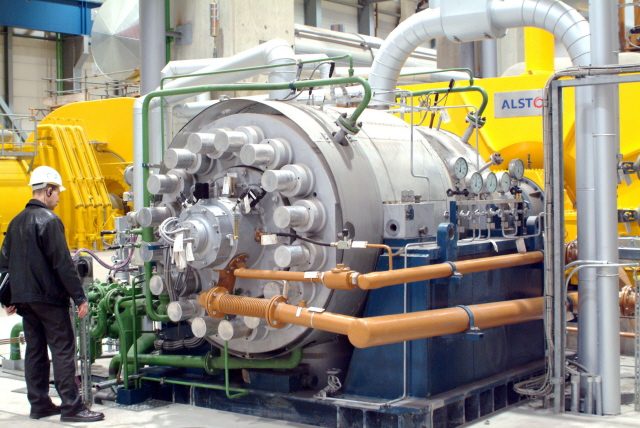
A pump from the manufacturer ksb delivering $2500 t/h$ of water at 350 bar in a steam power plant. Liquid pumps are usually powered by an electric motor, but this model is mechanically driven by the turbine and must therefore operate over a wider speed range. Its maximum power is $38 MW$; the power of the driven turbine exceeds $800 MW$. — Figure 9.2:A pump from the manufacturer ksb delivering $2500 t/h$ of water at 350 bar in a steam power plant. Liquid pumps are usually powered by an electric motor, but this model is mechanically driven by the turbine and must therefore operate over a wider speed range. Its maximum power is $38 MW$ ; the power of the driven turbine exceeds $800 MW$ .

Photo CC-by-sa KSB Aktiengesellschaft, Frankenthal

The specific power required to compress a fluid flow from a pressure $p_{\mathrm{A}}$ to a pressure $p_{\mathrm{B}}$ , in a reversible process, is expressed from the relation 3/22. Since the specific volume $v_{L}$ of pure saturated liquid water (approximately $v_{L}= 1 \times 10^{-3}m^{3}kg^{-1})$ varies very little with its pressure, we can write:

w_{\mathrm{liquid} \mathrm{pump}}\approx v_{L}\int _{\mathrm{A}}^{\mathrm{B}} dp = v_{L}(p_{\mathrm{B}}- p_{\mathrm{A}})

(9/4)

in the case of an approximately reversible pump operating with liquid water.

Example 9.1

In a power plant, a pump is fed with a mass flow of $35 kg s^{-1}(77.2 lb/s)$ of liquid saturated water at $0.5 bar (7.25 psi)$ . The water is compressed in an approximately isentropic manner until $40 bar (580.2 psi$ . What is the required power?

The process can be drawn qualitatively on a temperature-entropy diagram as shown below.

In Steam Table 3 at $0.05 MPa$ we read the inlet enthalpy $h_{\mathrm{A}}= h_{L0.05 MPa}= 340.5 kJ kg^{-1}$ . The specific volume will remain almost constant in the pump, at the value $v_{\mathrm{A}}= v_{L0.05 MPa}= 0.001 03 m^{3}kg^{-1}$ .

Using equation 9/4 we calculate $\dot{W}_{\mathrm{pump}}\approx \dot{m} v_{L}(p_{\mathrm{B}}- p_{\mathrm{A}}) = 35 \times 0.001 03(40 \times 10^{5}- 0.5 \times 10^{5}) = +142.4 kW$ .

Since the compression is assumed to be isentropic, we could also start from the fact that $s_{\mathrm{A}}= s_{\mathrm{B}}$ to obtain $h_{\mathrm{B}}$ by interpolation in Steam Table 1 and thus calculate the power of the pump. A calculation of $v_{\mathrm{B}}$ using this method allows us to see that the specific volume varies imperceptibly (less than $0.1 \%)$ during this process.

Since we have calculated the pump power, we are able to calculate $h_{\mathrm{B}}=\dot{} \frac{W_{\mathrm{pump}}}{m} + h_{\mathrm{A}}= 482.9 kJ kg^{-1}$ , which is the enthalpy of the water at the boiler inlet, a very useful information for later calculating the boiler power.

9.3.3 Boiler¶

In steam power plants, heat inputs occur at constant pressure. The water in the thermodynamic cycle is heated by contact with another pipeline: air in the case of combustion plants (waste, coal, gas), or water from a secondary circuit in the case of nuclear power plants (where the secondary circuit is used to avoid passing the high-pressure water from the thermodynamic cycle directly through the reactor core).

The wondrous behavior of fluids when they change phase works to our advantage here: in two-phase mixtures, a process at constant pressure also occurs at constant temperature (§5.2.2), allowing us to approach the conditions prescribed by Carnot without the need for any moving parts.

Because it operates at high pressure (beyond 60 bar in modern power plants) and is the scene of significant heat transfer and temperature gradients, the boiler is an expensive and heavy component (figures 9.3 and 9.4), even though its operating principle is simple.

When the heat in the power plant comes from combustion, the thermal energy of the gases can only be transferred to the water in the circuit when the temperature of the water is lower. Thus, the higher the minimum temperature of the water, and the greater the amount of heat lost above the boiler. The efficiency $\eta _{\mathrm{boiler}}= \frac{Q_{\mathrm{water}}}{Q_{\mathrm{heat} \mathrm{source}}}$ of a high-performance gas boiler is typically around $80 \%$ .

Since no work is supplied in the boiler, the power $\dot{Q}_{\mathrm{boiler}}$ supplied to the water by the boiler is expressed as:

Q_{\mathrm{boiler}}=\dot{m} (h_{2}- h_{1})

(9/5)

The difference in density between the two phases in the boiler makes it difficult to superheat the steam in the presence of liquid (the liquid, being

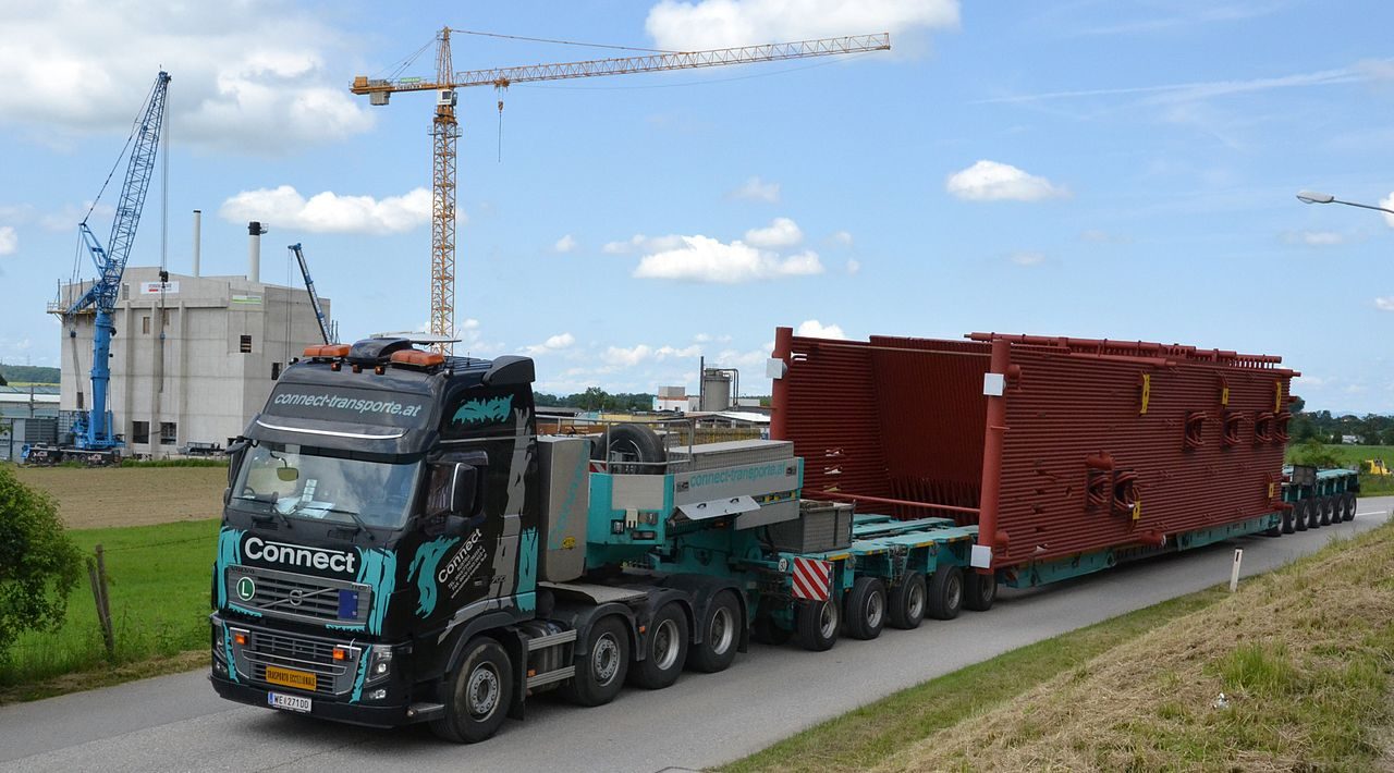
Figure 9.3:Transport of the boiler for a wood power plant capable of withstanding a pressure of 100 bar.

Photo CC-by-sa by Commons User:Sensenschmied

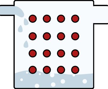
Figure 9.4:Schematic representation of a fire-tube boiler. Water enters in the liquid state on the left and exits at the top right in the form of saturated steam. In *fire-tube boilers*, the gas pipes pass through the heat exchanger filled with water. In more recent *water-tube boilers*, it is the water pipes that pass through the heat exchanger filled with hot gases. The latter technique is not detailed in this book, but its thermodynamic working principle is identical.

Diagram CC-by-sa by Olivier Cleynen denser and therefore at the bottom of the boiler, is more likely to absorb heat at high temperature). We will therefore always consider that the water is in the form of saturated vapor (index $V)$ at the outlet of the boiler.

9.3.4 Turbine¶

The turbine (figures 9.5 and 9.6) is the centerpiece of any steam power plant. Several tens of meters long in modern power plants, it is carefully balanced, installed in its casing, and, if given adequate attention (minimization of temperature gradients, advanced lubrication), can deliver mechanical power for several decades without any interruption.

The efficiency of a turbine is measured by comparing its power with that of an ideal turbine (a turbine that would be isentropic). We call this parameter the isentropic efficiency $\eta _{\mathrm{T}}$ :

\eta _{\mathrm{T}}\equiv \frac{\dot{W}_{\mathrm{actual} \mathrm{turbine}}}{\dot{W}_{\mathrm{isentropic} \mathrm{turbine}}}

(9/6)

where $\dot{W}_{\mathrm{actual} \mathrm{turbine}}$ is the actual power supplied by the turbine, and $W_{\mathrm{isentropic} \mathrm{turbine}}$ is the power of an isentropic turbine operating with the same mass flow rate and between the same pressures.

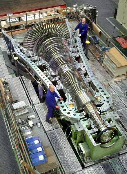
Figure 9.5:Turbine of a medium-sized steam power plant. As the water passes through the turbine, it loses energy in the form of work and its specific volume increases, requiring increasingly larger blades.

Photo CC-by-sa MAN SE

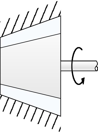
Figure 9.6:Schematic representation of a steam turbine.

Diagram CC-by-sa by Olivier Cleynen

The actual power is expressed in terms of the properties of the fluid at the inlet and outlet of the turbine:

W_{\mathrm{actual} \mathrm{turbine}}=\dot{m} (h_{2 \mathrm{actual}}- h_{1}) =\dot{m} \eta _{\mathrm{T}}(h_{2^{'}}- h_{1})

(9/7)

We use equation 9/7 to predict the state of the steam at the outlet of any turbine whose power and isentropic efficiency are known.

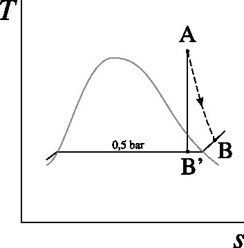
An important parameter that must be monitored is the dryness fraction of the water, especially in the final stages. Indeed, as we have already seen in section §5.4.5 p. 138, the isentropic curves always end up crossing the saturation curve: in an isentropic expansion, the steam always ends up condensing. The liquid droplets, much denser than the steam surrounding them, then violently impact the blades, causing erosion. The thermodynamic engineer will therefore ensure to maintain a high dryness fraction, typically not dropping below $95 \%$ .

Example 1

We start by imagining that we are equipped –a thermodynamicist’s irrepressible dream!– with an isentropic turbine between these same pressures. In Steam Table 1 at $4 MPa$ , we read $h_{\mathrm{A}}= 3674.9 kJ kg^{-1}$ and $s_{\mathrm{A}}= 7.3705 kJ K^{-1}kg^{-1}$ . The steam at the outlet of this hypothetical turbine (at B’) has the same entropy: $s_{\mathrm{B}^{'}}= s_{\mathrm{A}}$ , and we observe that $s_{\mathrm{B}^{'}}< s_{V0.05 MPa}$ : the water is partially condensed. The calculation of the dryness fraction (§5.3.3) allows us to calculate the value of its enthalpy: $h_{\mathrm{B}^{'}}= h_{L0.05 MPa}+ ^{s_{\mathrm{B}'}-s_{L0.05 MPa}}_{s_{LV0.05 MPa}}h_{LV0.05 MPa}= 2566.3 kJ kg^{-1}$ .

We can now return to the the painful reality: the actual turbine delivers only $85 \%$ of the power of this hypothetical turbine, so $\dot{W}_{\mathrm{real} \mathrm{turbine}}=\dot{} m\eta _{\mathrm{T}}(h_{\mathrm{B}^{'}}-h_{\mathrm{A}}) = 35\times 0.85\times (2566.3\times 10^{3}-3674.9\times 10^{3}) = -32 980 kW = -32.98 MW$ .

Equation 9/7 allows us to calculate the enthalpy $h_{\mathrm{B}}$ actually obtained at the outlet of the turbine: $h_{\mathrm{B}}=\dot{} \frac{W_{\mathrm{turbine}}}{m} +h_{\mathrm{A}}= 2732.6 kJ kg^{-1}$ , which is very useful for later calculating the power of the condenser. A glance at Steam Table 2 shows us that $h_{\mathrm{B}}> h_{V0.05 MPa}$ : the steam is dry throughout its expansion.

The $15 \%$ of missing power in the mechanical shaft of the turbine is transferred as heat (through turbulence) to the water during its expansion in the turbine.

The power of the turbine is two hundred times greater than the power supplied to the pump in example 9.1 on page 245 between these same pressures.

9.3.5 Condenser¶

The condenser (figures 9.7, 9.8 and 9.9), the least glorious component of the power plant, is responsible for rejecting all the heat that the engineer no longer knows how to use (§7.2). The water is always cooled at constant pressure, which does not require any moving parts.

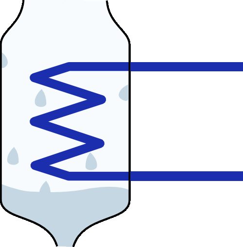
Figure 9.7:Schematic representation of a condenser. Water from the thermodynamic cycle enters at the top, in a state close to saturated vapor. It exits at the bottom in the liquid state. The heat extraction is usually ensured by a secondary water circuit (illustrated in dark blue) which is in contact with the atmosphere.

Diagram CC-by-sa Olivier Cleynen

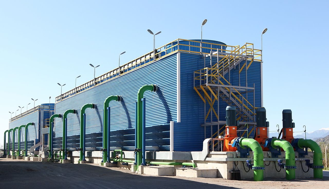
Figure 9.8:A condenser in which the heat is dissipated directly into the atmosphere, by forced convection using fans.

Photo CC-by-sa Cenk Endustri

Technologically, the condenser is a simple element: the steam pipeline is simply brought into contact with a low-temperature circuit. Usually, this cooling circuit consists of external water from a river or the sea, which is then itself cooled by evaporation in the large towers seen around power plants. Using a secondary cooling circuit has two benefits. Firstly, the pressure in the condenser can be lowered to a level lower than atmospheric pressure, thereby reducing the minimum temperature of the cycle. Secondly, the water from the thermodynamic cycle, purified at considerable effort, is not lost to the atmosphere.

Since the pressure of the steam inside the condenser is often very low (down to 0.1 bar or $0.15 psi)$ so as to reduce the minimum temperature of the power plant cycle, care must be taken to ensure the tightness of the condenser to prevent external air or water from entering the main circuit.

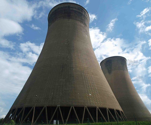
Cooling towers of the Eggborough coal power plant (1967, 1960 MW) in the United Kingdom. In these towers, the heat extracted from the water in the condenser is dissipated into the atmosphere. This cooling is done through a secondary water circuit, which is brought into contact with the atmosphere and partially evaporates. — Figure 9.9:Cooling towers of the Eggborough coal power plant (1967, $1960 MW$ ) in the United Kingdom. In these towers, the heat extracted from the water in the condenser is dissipated into the atmosphere. This cooling is done through a secondary water circuit, which is brought into contact with the atmosphere and partially evaporates.

Photo CC-by-sa Steve Fareham

The power rejected by the steam in the condenser is expressed as:

\dot{Q}_{\mathrm{condenser}}=\dot{m} (h_{2}- h_{1})

(9/8)

9.4 Steam Engine Cycles¶

9.4.1 The Carnot cycle¶

Since the Carnot cycle which we studied in §7.3 serves as a reference in the design of engines, we start our study with it. The temperature of a liquid-vapor mixture remains constant when heated at constant pressure, so achieving isothermal heat transfers (an important characteristic of the Carnot cycle) is relatively easy with steam. A steam engine based on a Carnot cycle is schematized in figures 9.10 and 9.11.

The efficiency of the Carnot engine cycle (7/6) is only reached if the turbine and compressor operate isentropically. In practice, as we have seen, the power of the turbine is always lower, and that of the compressor always higher, than if they were isentropic.

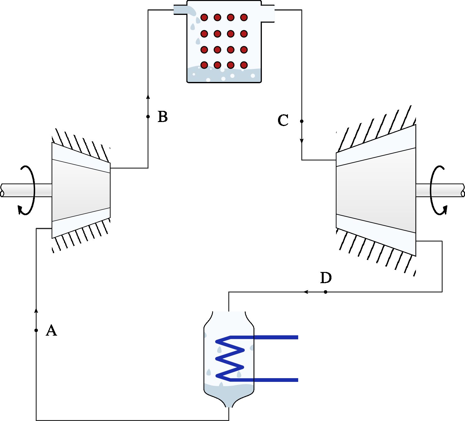
Figure 9.10:Diagram of a steam power plant operating on a Carnot cycle.

Diagram CC-by-sa Olivier Cleynen

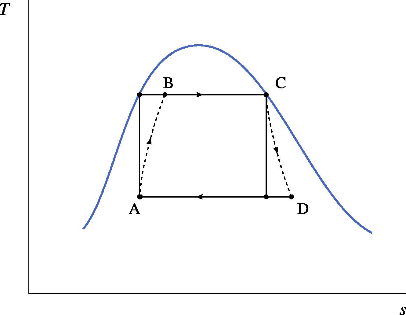
Figure 9.11:Temperature-entropy diagram of a steam power plant operating on a Carnot cycle. The dashed paths represent the real (irreversible) processes of the fluid during compressions and expansions.

Diagram CC-0 Olivier Cleynen

9.4.2 The Rankine cycle¶

In practice, using the Carnot cycle as described above poses several difficulties:

• Compressing a two-phase mixture is challenging (§9.3.2 p. 244);

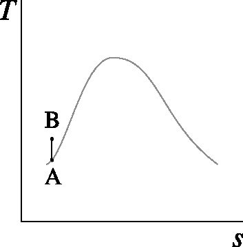
• In the condenser, it is difficult to stop condensation at a specific point (point A in figures 9.10 and 9.11 above), where the dryness fraction is close but not equal to zero).

In 1859, English engineer William Rankine proposed a modification of the cycle by continuing the condensation until saturation and by compressing the water only in the liquid state. A machine based on this cycle is described in figures 9.12 and 9.13.

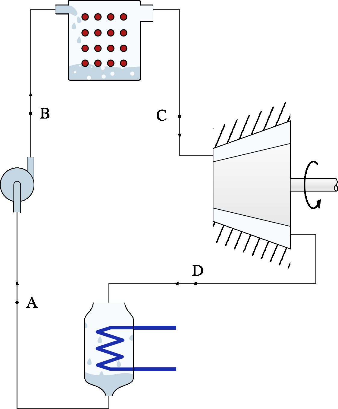
Figure 9.12:Diagram of a steam power plant operating on a Rankine cycle. The water at the outlet of the condenser is in the form of saturated liquid; it enters the boiler at a lower temperature.

Diagram CC-by-sa Olivier Cleynen

The Rankine cycle thus uses a liquid water pump instead of a compressor dealing with a liquid-vapor mixture. Technologically, a pump is simpler to design, manufacture, and operate than a compressor. Another advantage is that compressing a liquid is several tens of times more energy-efficient than compressing a mixture (§9.3.2).

This energy saving, however, is not without consequence: at the outlet of the pump (point B), the water is at a much lower temperature than it was at the outlet of the compressor in figure 9.10. It is the boiler that will have to return the water to the state of saturated liquid. In other words, a considerable additional expenditure of heat must be supplied to compensate for the decrease in compression power.

It can be noticed that a significant part of the heat supplied by the boiler (that is, $q_{\mathrm{boiler}}= h_{\mathrm{C}}- h_{\mathrm{B}})$ is no longer supplied at the maximum temperature of the cycle. We saw in chapters 7 and 8 that supplying heat at low temperature always results in a lower efficiency.

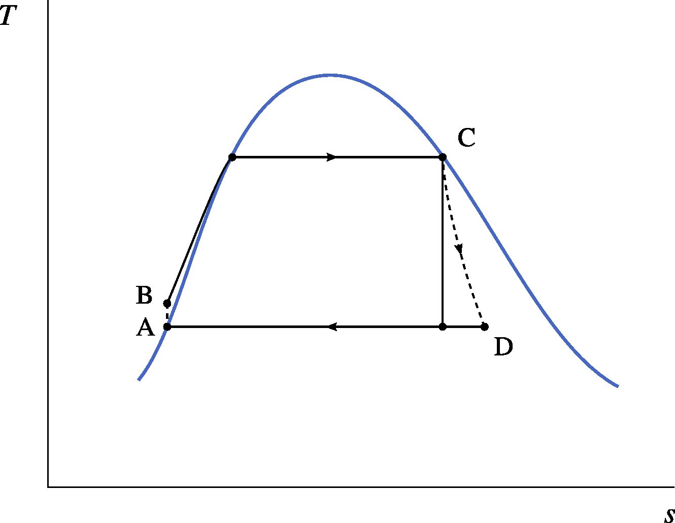
Figure 9.13:Temperature-entropy diagram of a steam power plant operating on a Rankine cycle.

Diagram CC-0 Olivier Cleynen

However, in practice, this heat input can make it possible to exploit low-temperature heat sources, such as exhaust gases that were previously discharged above the boiler. Thus, in some cases, the drop in thermodynamic efficiency $(\eta _{\mathrm{engine}})$ can be compensated by an increase in the boiler efficiency $(\eta _{\mathrm{boiler}})$ , which can extract more energy from the fuel to transfer it to the steam.

Rankine thus deliberately deviated from the Carnot cycle and, in doing so, reduced the thermodynamic efficiency (although this decrease can often be offset by an increase in boiler efficiency). On the other hand, by eliminating the compressor, his modification greatly reduces the size and complexity of the machine.

9.4.3 Superheating¶

In order to reduce the specific steam consumption (ssc, see §9.2.2 p. 242) of a power plant, it is desirable to increase the power delivered by the turbine for a given steam flow rate. To achieve this, there are several options:

• Increase the enthalpy at the inlet of the turbine (in other words, increase the saturation pressure in the boiler). Unfortunately, this requires the boiler to be more resistant and more expensive; moreover, it reduces the amount of specific heat that can be supplied in it, since the enthalpy of vaporization $h_{LV}$ decreases with temperature;

• Reduce the enthalpy at the outlet of the turbine (in other words, decrease the pressure in the condenser). This requires a larger turbine, promotes the entry of air bubbles into the steam circuit, and above all, reduces the steam dryness fraction at the turbine outlet;

• Increase the enthalpy (and thus the temperature of the steam) after its exit from the boiler.

This allows for fully utilizing the turbine’s capacities, whose metallurgical limits (generally around $1000 K)$ often already exceed those of the boilers.

It is this last option that is very often chosen. This modification is called superheating: the steam is superheated at the outlet of the boiler, at constant pressure, through a series of tubes heated to a higher temperature (figures 9.14 and 9.15). Superheating could theoretically be done in the boiler itself; however, since the density of dry steam is relatively low, it is easier to bring it in contact with the hottest gases outside (and below) the boiler.

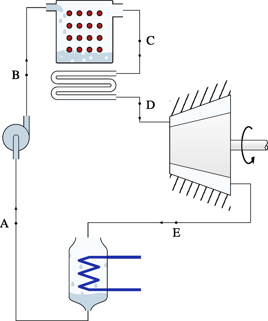
Diagram of a steam power plant operating on a superheated Rankine cycle. The water at the outlet of the boiler is heated to a higher temperature (section C $\rightarrow$D) before entering the turbine. — Figure 9.14:Diagram of a steam power plant operating on a superheated Rankine cycle. The water at the outlet of the boiler is heated to a higher temperature (section C $\rightarrow$ D) before entering the turbine.

Diagram CC-by-sa Olivier Cleynen

The main advantage of this modification is that it allows for a reduction in specific consumption that is relatively simple to implement. Additionally, increasing the average temperature at which heat is supplied tends to increase thermodynamic efficiency. Finally, it becomes possible to shift the operating range of the turbine entirely into the realm of dry steam: erosion of the blades by liquid water is thus avoided. All modern steam power plants now use a superheating circuit.

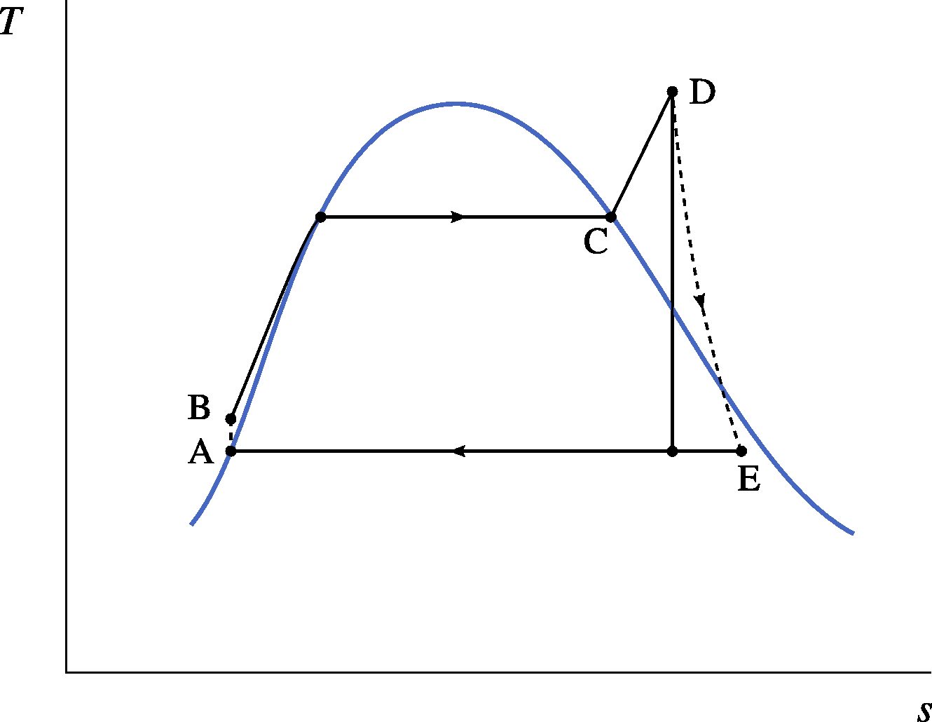
Figure 9.15:Temperature-entropy diagram of a steam power plant operating on a superheated Rankine cycle.

Diagram CC-0 Olivier Cleynen

9.4.4 Reheat¶

In order to again increase the power of the machine without increasing the steam flow rate (and therefore its overall size and the cost of the boiler), it is possible to heat the steam a second time before its exit from the turbine (figures 9.16 and 9.17). This is called reheat.

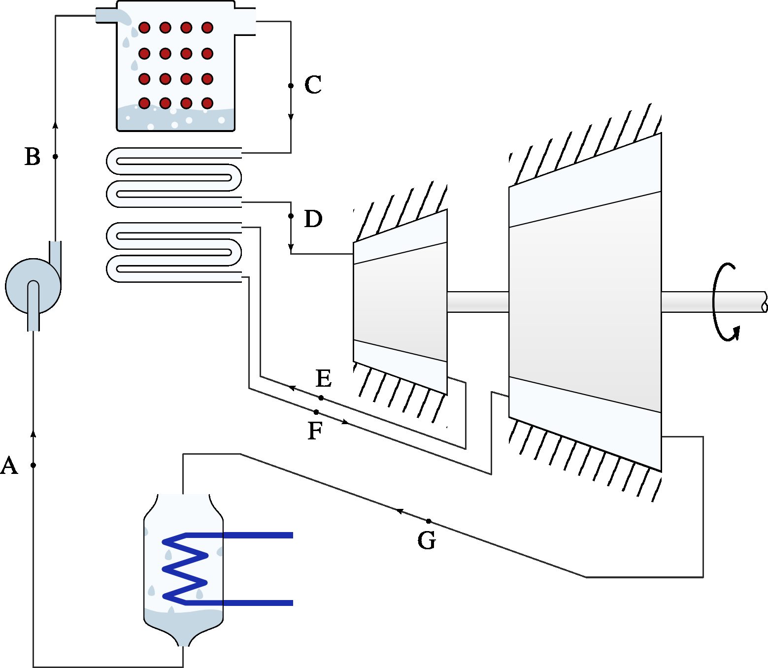
Figure 9.16:Diagram of a steam power plant operating on a reheated Rankine cycle.

Diagram CC-by-sa Olivier Cleynen

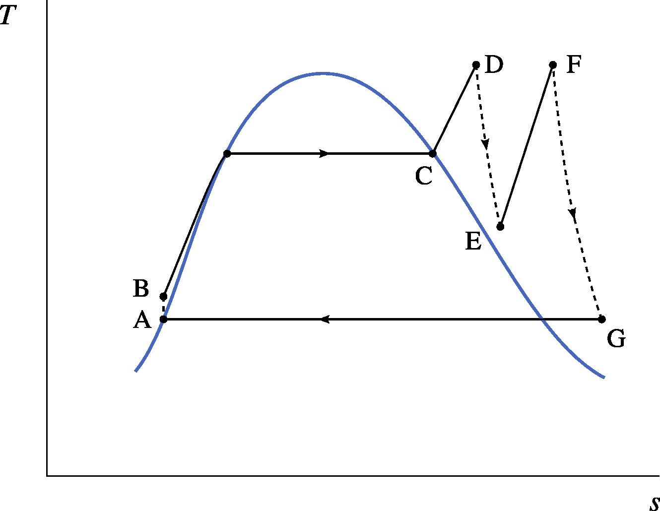
Figure 9.17:Temperature-entropy diagram of a steam power plant operating on a reheated Rankine cycle.

Diagram CC-0 Olivier Cleynen

With this modification, the expansion in the turbine is interrupted, and the steam is led into a new series of tubes to raise its temperature back to a high level (usually to the metallurgical limits of the turbine). The expansion is then finally completed down the condenser pressure.

Providing that the average heating temperature is increased, the overall efficiency of the power plant is increased too; therefore, the choice of the reheat pressure matters. The specific consumption is reduced in all cases, with the advantages described above.

9.4.5 Regeneration¶

When Rankine modified the Carnot cycle, he reduced the work required to compress the water and increased the heat necessary to bring it to the turbine inlet. However, the thermodynamic efficiency went down: indeed, the water temperature at the boiler entry was reduced. The reversibility of the heat transfer was thus reduced.

In order to increase the reversibility of the cycle (and therefore its efficiency), it is possible to gradually heat the water, using the heat from the turbine (where the steam temperature varies). This technique is called regeneration. One can imagine a cycle as described in figures 9.18 and 9.19 below, where the liquid water at the pump outlet is gradually heated by cooling the turbine.

In the limit case where all the heat used during regeneration is transferred with an infinitely small temperature difference, the cycle is reversible and the Carnot engine efficiency is reached even if one does not strictly follow the Carnot cycle.

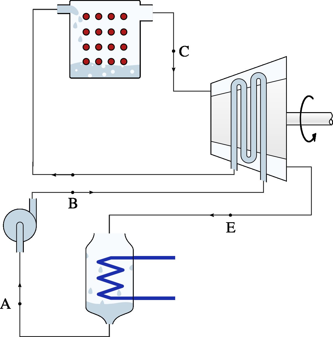
Diagram of a steam power plant with regeneration. Heat is extracted from the turbine to heat the liquid water before it enters the boiler. Ideally, heat transfer is reversible. — Figure 9.18:Diagram of a steam power plant with regeneration. Heat is extracted from the turbine to heat the liquid water before it enters the boiler. Ideally, heat

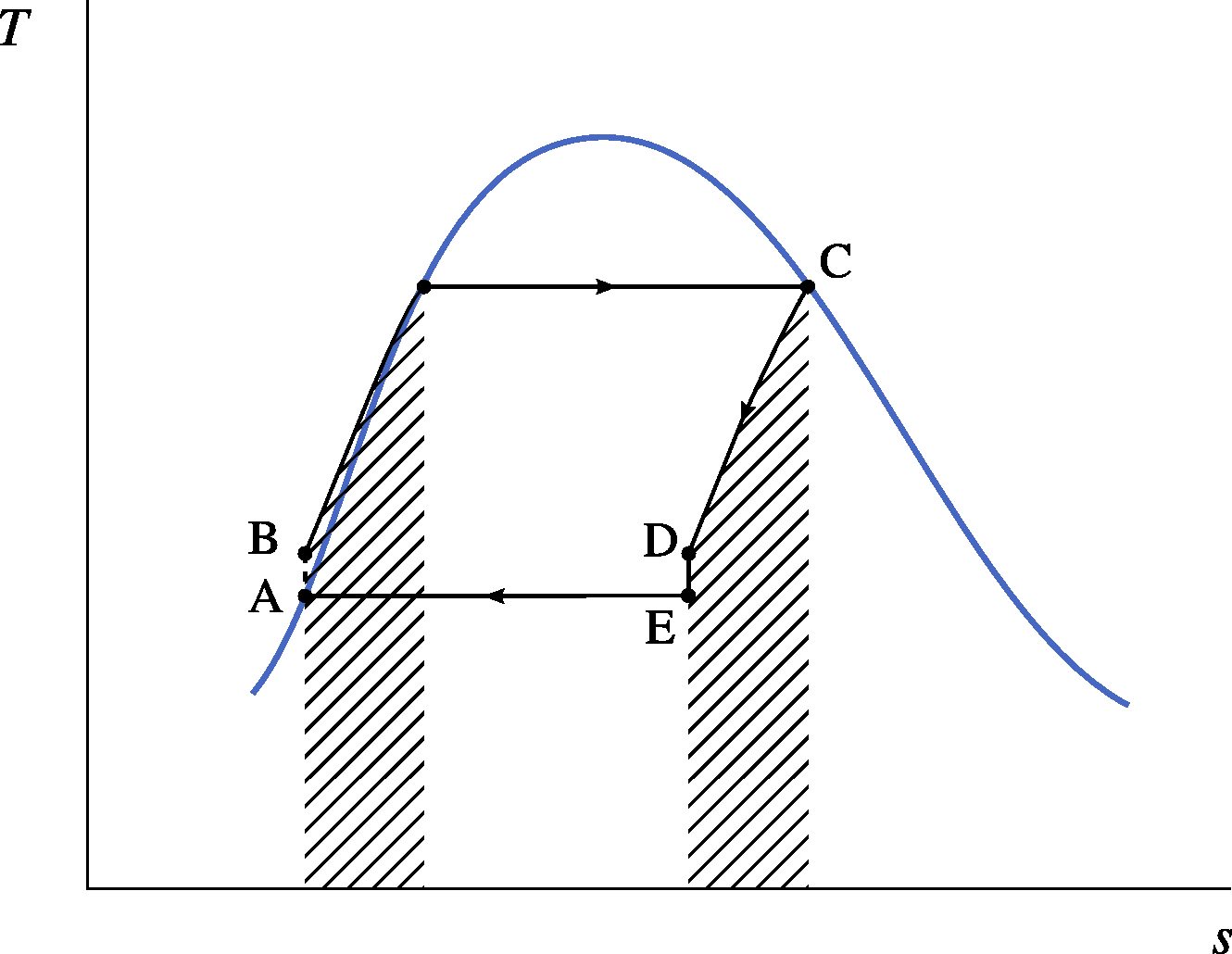
transfer is reversible. ^{\mathrm{Diagram} \mathrm{CC-by-sa} \mathrm{Olivier} \mathrm{Cleynen}}

(1)

Figure 9.19:Temperature-entropy diagram of a steam power plant with regeneration.

Diagram CC-0 Olivier Cleynen

In practice, such a device is difficult to implement, because it requires adding a non-uniform-temperature cooling system to the turbine, an element whose design and manufacturing are already very costly. Moreover, cooling the steam reduces its dryness fraction, increasing the amount of liquid water eroding the turbine components.

In order to implement regeneration, the turbine bleed technique is used. Steam is drawn off from the turbine and mixed with the liquid feedwater at the pump outlet (figures 9.20 and 9.21). This results in a heat transfer that is easier to implement.

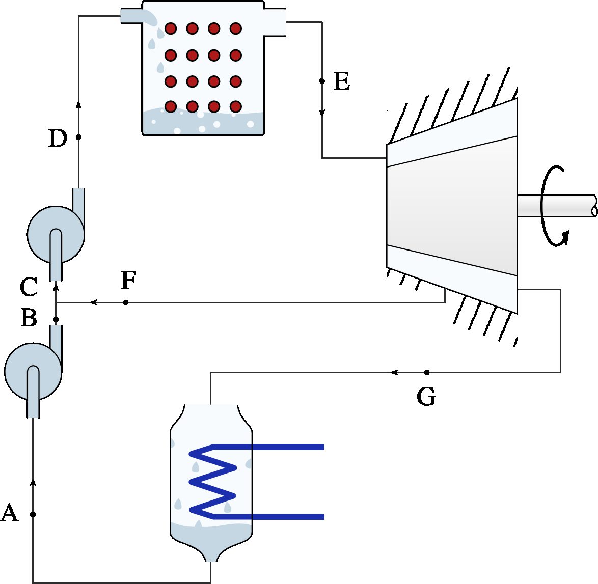
Figure 9.20:Diagram of a steam power plant with steam bleed. The steam prematurely extracted from the turbine is used to heat the liquid water during pumping.

Diagram CC-by-sa Olivier Cleynen

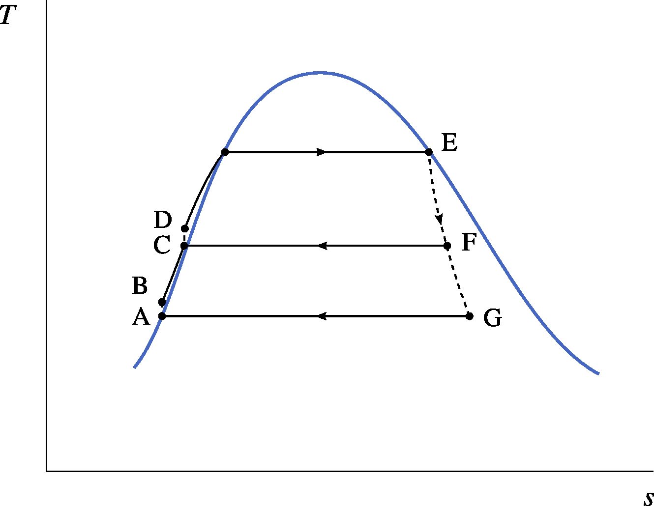
Figure 9.21:Temperature-entropy diagram of a power plant with steam bleed.

Diagram CC-0 Olivier Cleynen

In practice, many bleeds (sometimes called steam extractions) are performed in steam power plant circuits in order to control the heat flows (figure 9.22). They also allow, through discharge valves, to precisely regulate turbine mass flows and thus quickly adjust the power of the plant to the demand.

Diagram CC-by-sa Olivier Cleynen

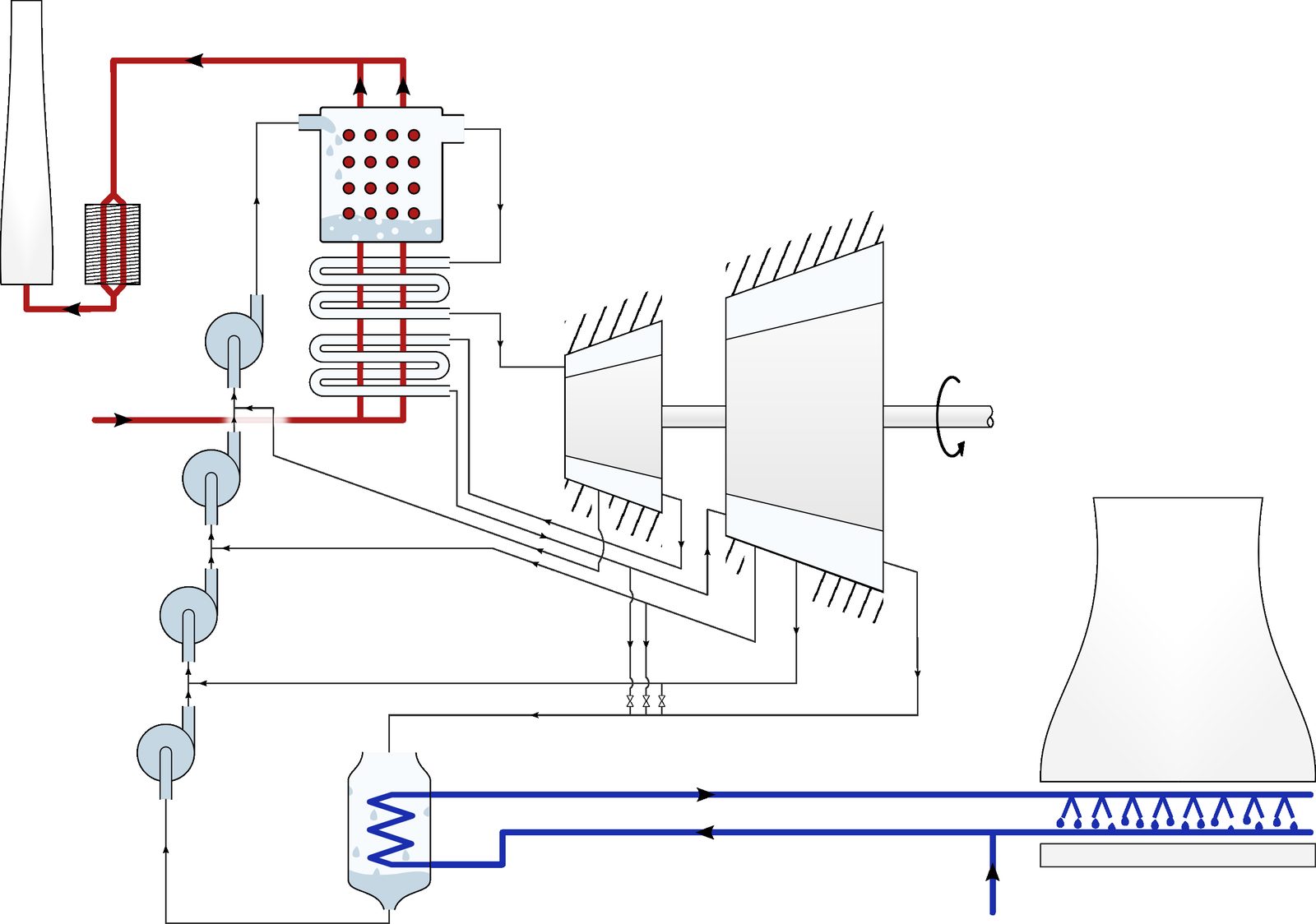
Figure 9.22:A steam power plant circuit combining superheating, reheat, regeneration, and discharge ducts. It is left to the curious student the pleasure of tracing the processes on a temperature-entropy diagram, and imagining themselves at the controls of the machine supplying their coffee maker with electricity.

A Bit of History

From the Steam Turbine to the Gas Turbine

At the beginning of the 20th century, the turbine replaced pistons and cylinders in all steam engines. A turbine has a complex geometry, sensitive to manufacturing imperfections, making its construction more delicate than that of cylindrical pistons. In return, it makes for an engine with simple arrangement, little vibration, and with easier assembly, maintenance, and lubrication, allowing for increased power or reduced volume. The Anglo-Irish engineer Charles Parsons dramatically demonstrated this in 1897 with the Turbinia (figure 9.23), the first ship of its kind, which was so fast that no military vessel could catch up with it. Ten years later, the entire Royal Navy had switched to turbines for ship propulsion.

Developing a gas turbine engine is much more challenging than for steam. Certainly, air (or burnt gases) and dry steam have very similar properties: thus a steam turbine works very well with compressed air. The difficulty lies at the other end of the engine. In steam engines, compressing water is done in the liquid state, which is very efficient. Compressing water at $10^{\circ}C$ from 1 to 10 bar, for example, only requires

w_{\mathrm{A}\rightarrow \mathrm{B}}\approx v_{L}(p_{\mathrm{B}}-p_{\mathrm{A}}) = 0.001(10-1)\times 10^{5}= 900\,J\,kg^{-1}

(2)

(equation 9/4). In contrast, doing the same with air requires a minimum specific power of

w_{\mathrm{A}\rightarrow \mathrm{B}}= c_{p}\Delta T = c_{p}\bigl(T_{\mathrm{A}}(p_{\mathrm{B}}/p_{\mathrm{A}})^{\frac{\gamma-1}{\gamma}}- T_{\mathrm{A}}\bigr) = 1005 \bigl(283.15 \times 10^{\frac{0.4}{1.4}}- 283.15\bigr) = 265\,kJ\,kg^{-1}

(3)

(equations 4/34 and 4/37), almost three hundred times more!

Figure 9.23:The Turbinia, Charles Parsons’ yacht used as a demonstrator for his research in maritime propulsion. With its three steam turbines and nine propellers, it reached $60 km/h$ and allowed its owner to ridicule the Royal Navy during Queen Victoria’s jubilee parade in 1897.

Photo by Alfred John West, 1897 (public domain)

In the realm of air-based engines, the situation was quite different: until the late 1930s, all engines were piston-cylinder based. Piston technology peaked in the aeronautical sector, where cylinders were arranged in a star pattern behind the propellers to reduce bulkiness and vibrations. In these machines, such as the Twin Wasp by Pratt & Whitney, the mechanical arrangement of cylinders, connecting rods, and crankshafts was absolutely phenomenal (figure 9.24), and the intake and exhaust systems going to and back from dozens of combustion chambers were labyrinthine.

Figure 9.24:Cross-section of a Pratt & Whitney Twin Wasp engine (1932), showing the internal arrangement with connecting rods and crankshafts connecting the two rows of seven pistons arranged in a star pattern. The engine, with a displacement of $30 L$ , produced over $1000 hp$ and was produced in over $170 000$ units.

Photo CC-by-sa Olivier Cleynen

We saw in §9.4.2 that using liquid compression is not without consequences – it must be compensated by greater power at the boiler and reduces the thermodynamic efficiency – but it greatly facilitates the development of the engine. Since almost all of the net power of the engine comes from the turbine, a highly irreversible or incomplete expansion only affects the power and efficiency of the engine. In a gas turbomachine, on the other hand, the turbine also powers the compressor: it plays a dual role. For as long as it does not supply enough power to match that of the compressor, the engine will not run at all. The isentropic efficiency of the turbine and compressor thus become paramount parameters (we will revisit this in §10.2.2 with the concept of work ratio) and it follows that the development of a gas turbomachine is an ambitious undertaking.

Both Whittle and von Ohain focused their efforts on an ingenious aeronautical engine called turbojet: it is the exhaust gases, in large quantities and with high residual pressure, that would provide the engine’s thrust (§10.5.3). The operating principle is very simple (the air flows in a steady state and there is only one moving part) but the challenges were numerous. Like an aircraft wing, the compressor blades tend to stall at low power and during transient phases, causing abrupt and destructive flow changes. In the combustion chambers, it is necessary to prevent the flame from impinging on the walls (which would cause them to melt) or from extending, especially during ignition or reignition, into the turbine. Weight constraints require the use of lightweight materials which complicate manufacturing. The two engineers carried out their work in the heart of the Second World War, each funded by military budgets, and the first jet aircraft flew in 1940. The subsequent production aircraft were delicate to operate, unresponsive, and their service life barely reached 20 hours. They arrived too late and in insufficient numbers to affect the course of the conflict.

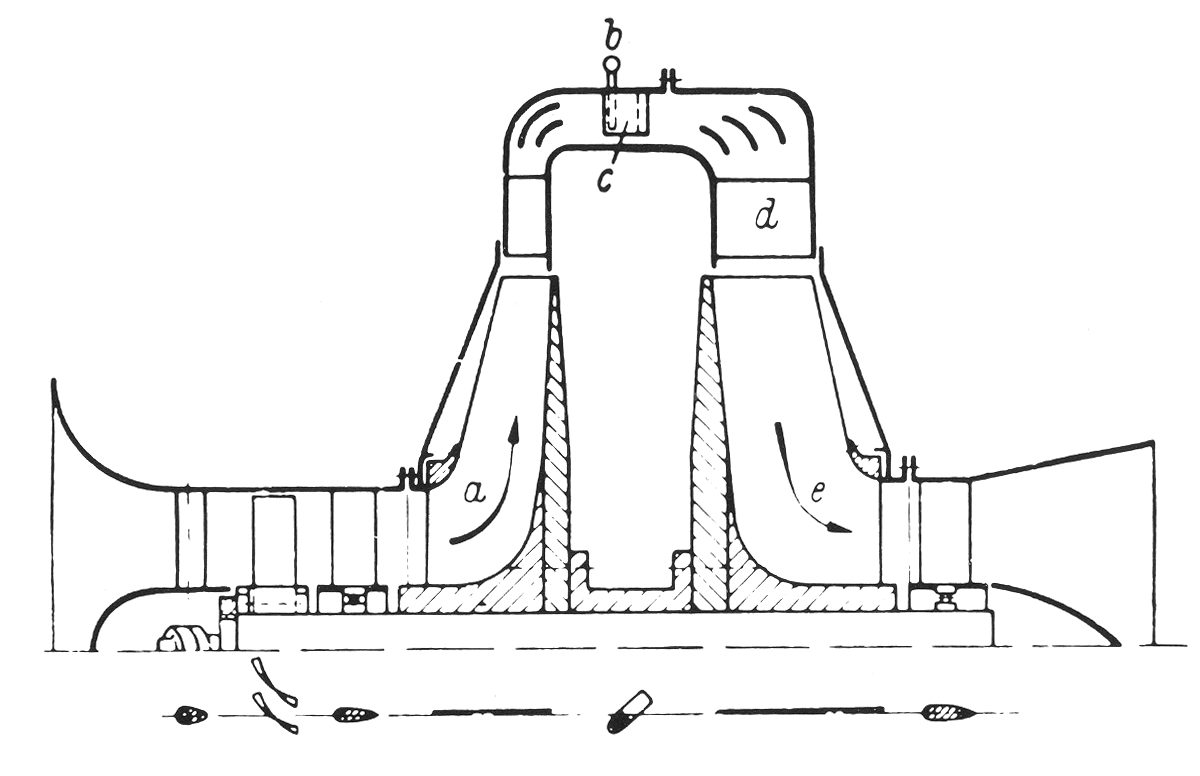
Cross-sectional diagram of the Heinkel He S-1, the first prototype tested by Hans von Ohain in 1937. The compressor consists of an axial stage and a centrifugal stage; the turbine is centripetal. There is only one moving part and its speed is invariant. — Figure 9.25:Cross-sectional diagram of the *Heinkel He S-1*, the first prototype tested by Hans von Ohain in 1937. The compressor consists of an axial stage and a centrifugal stage; the turbine is centripetal. There is only one moving part and its speed is invariant.

Diagram USAF (public domain)

At the end of the war, there was a surge of enthusiasm: aviation embraced the engine it had been waiting for over three decades. To understand why the jet engine became the Holy Grail of 20th century aeronautics, a bit of flight mechanics is needed. In subsonic flight, a well-designed aircraft has a drag

coefficient $C_{D}\equiv F_{D}\div \left(\frac{1}{2} A_{\mathrm{ref}.}\rho C_{\mathrm{flight}}^{2}\right)$ that is almost constant. Thus, when reducing the reference area

$A_{\mathrm{ref}.}$ of the wing surface and the ambient density $\rho$

(by gaining altitude), the flight speed $C_{\mathrm{flight}}$ can be increased while keeping the drag $F_{D}$ constant. The energy cost of moving the aircraft remains constant

– however, the required power $\dot{W}_{\mathrm{engine}}= F_{x}C_{\mathrm{flight}}$ increases proportionally to the speed. These characteristics make aircraft relatively energy-efficient machines, but very power-hungry, since they need to maintain the same thrust at very high speeds.

The jet engine had two advantages to address this issue. Firstly, it was compact, lightweight, and vibration-free, which is highly desirable for an application where drag (and thus the thrust to be provided) increases proportionally with the weight of the aircraft. Secondly, the propeller, which is very efficient at low speeds but with whose tips reach supersonic speeds early, thus limiting the speed of aircraft, was completely eliminated. Because of these qualities, the low efficiencies due to irreversible compressions and expansions, low pressure ratios, and excessively high gas speeds in the nozzles were acceptable.

Thus, the graceful Lockheed Constellation, the culmination of the era of propeller aviation, was instantly rendered obsolete by the arrival of the much faster De Havilland Comet in 1949, a remarkable quad-jet of the same size (figure 9.26). Even though it was initially unable to cover the same distance and it featured higher fuel consumption per kilometer, the Comet left no chance for its competitors. Its speed was an obvious quality for passengers, but also for the airlines, significantly increasing their productivity.

The Comet, after a serious design flaw was corrected, was itself surpassed by the Boeing 707 in 1957. Capable of flying further while carrying more payload, and even faster (at $900 km/h$ , the speed that all airliners have adopted since, the air on the wing’s upper surface barely reaches the speed of sound), the 707 marked the entry into the jet age, where airliners were no longer built by dozens but by thousands. Thus, in just twenty-five years, the gas turbine engine doubled the speed of aircraft and divided the price of tickets by four.

“Ready?” “Takeoff time!” The flight engineer pushes the throttle levers with me. NNggnniiiaavvrrooooooaaaaaaarrrrooouuummmmm... “N1s green.” It’s pushing hard, but accelerates ever so gently, given the weight of the behemoth. “Eighty knots” “Thrust set.” I have the tips of my feet on the rudder pedals, a precision similar to a kickboxing move. I’m enjoying every bit of it. 120 knots. I’m in control, guys. 432 passengers and 15 crew members are strapped in the back, ears and senses alert. 140 knots. Two bursts of light beacons pass by on the sides. The rudder, precise. “V1.” Another 20 knots to reach before the machine can fly. I can see end of the runway coming up, over there ahead. “Rotate.” At 170 knots, I pull gently, then more firmly. Five degrees of pitch. Ten degrees. It’s no longer rolling, the needle is at 185 knots. Twelve-degree pitch. Come on, my dear, we must climb. “Positive climb.” “Landing gear up.” The truth lies tonight between twelve and thirteen degrees of pitch, where the airspeed indicator needle comes to a standstill. We pass the hill, and three hundred feet below, the 747 flying by must feel like an earthquake.

Jacques Darolles, 1998

Le plus beau bureau du monde [42]

Nearly sixty years after the first flight of the 707, airliners still fly at the same speed, but jet engine technology has continued to advance [47]. With their carbon-epoxy or blown titanium fan blades, turbine stators printed in ceramics, their multiple laser-drilled pneumatic turbine cooling circuits, their electronic control, diagnostic and remote monitoring systems, they slowly but surely continue to increase in efficiency. Reliability is also remarkable: a modern engine on average only experiences an in-flight failure every $200 000$ flight hours, and is separated from the aircraft for maintenance only every $20 000$ hours or $10 000$ flights. Will a new type of engine ever render the jet engine obsolete and propel aviation forward into a new era?

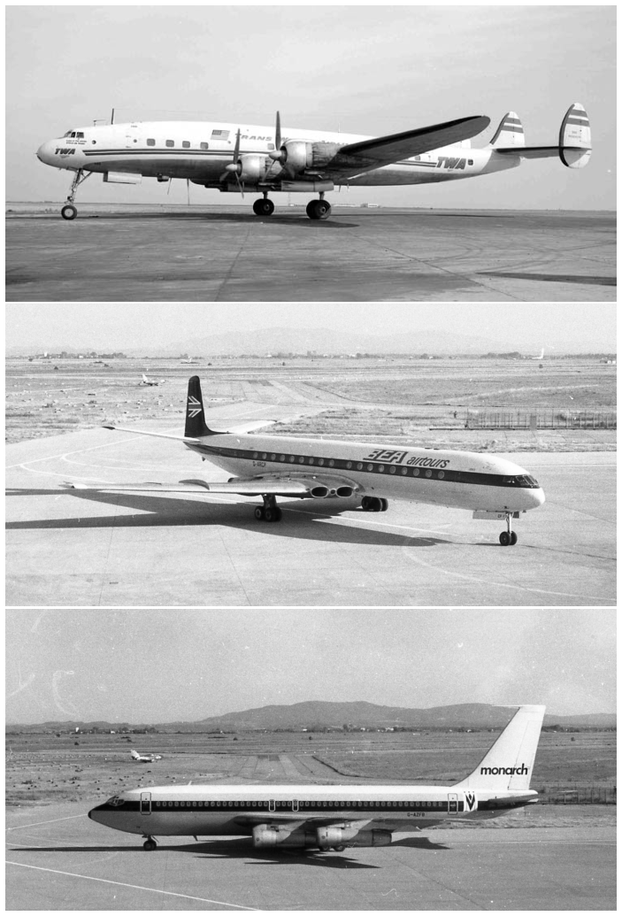
From top to bottom: The 1943 Lockheed Constellation, the culmination of the propeller aircraft era: four Wright Duplex-Cyclone supercharged 18-cylinder engines, capable of covering 3700 km (2300 mi) at 500 km/h (310 mph). The 1949 De Havilland Comet, the first jet airliner: four Halford Ghost turbojet engines, capable of covering 2400 km (1500 mi) at 740 km/h (460 mph). The 1957 Boeing 707, with a configuration and performances anticipating those of all its successors: four Pratt & Whitney JT3C turbojet engines, capable of covering 4300 km (2700 mi) at 900 km/h (560 mph). — Figure 9.26:From top to bottom:

Constellation Photo CC-by-sa by Bill Larkins

Comet Photo and 707 (edited) CC-by-sa by Piergiuliano Chesi

Problems¶

The properties of water are tabulated in Steam Tables 1, 2, and 3 (see Appendix A1 p. 305)

Air is considered an ideal gas.

$c_{v (\mathrm{air})}= 718Jkg^{-1}K^{-1} R_{\mathrm{air}}= 287Jkg^{-1}K^{-1}$

$c_{p (\mathrm{air})}= 1005Jkg^{-1}K^{-1} \gamma _{\mathrm{air}}= 1.4$

Exercise 9.1

Superheated Rankine cycle The Électricité de France power plant in Porcheville (figure 9.27) received heat from the combustion of oil, and used a steam cycle to power an electric generator. In the power plant, water cycled between the pressures of 0.1 and $140 bar (0.15$ and $2031 psi)$ . The steam reached $545^{\circ}C (1013 ^{\circ} F)$ , and the turbines had an isentropic efficiency of $80 \%$ . For the purposes of the problem, we consider that the cycle was based on a superheated Rankine cycle. 1. Sketch the physicalwater circuit in the power plant; draw the cycle followed on a temperature-entropy diagram, qualitatively (that is, without showing numerical values), showing the saturation curve. 2. What is the enthalpy of the water at the outlet of the turbines? 3. What is the enthalpy of the water at the outlet of the pumps? 4. What is the thermal efficiency of the power plant? 5. What is the specific steam consumption of the power plant, namely, the mass of steam that must enter the turbine for the installation to supply $1 kWh$ of work? Photo CC-0 Olivier Cleynen

Answer

See figures 9.14 and 9.15 p. 256; 2) With $s_{\mathrm{E}}= s_{\mathrm{D}}= 6.5399 kJ kg^{-1}$ and $\eta _{\mathrm{T}}= 80 \%$ , we obtain $h_{\mathrm{E}}= 2287.7 kJ kg^{-1}$ as in example 9.2 p. 249; 3) Using equation 9/4 we obtain $h_{\mathrm{B}}= 205.9 kJ kg^{-1}$

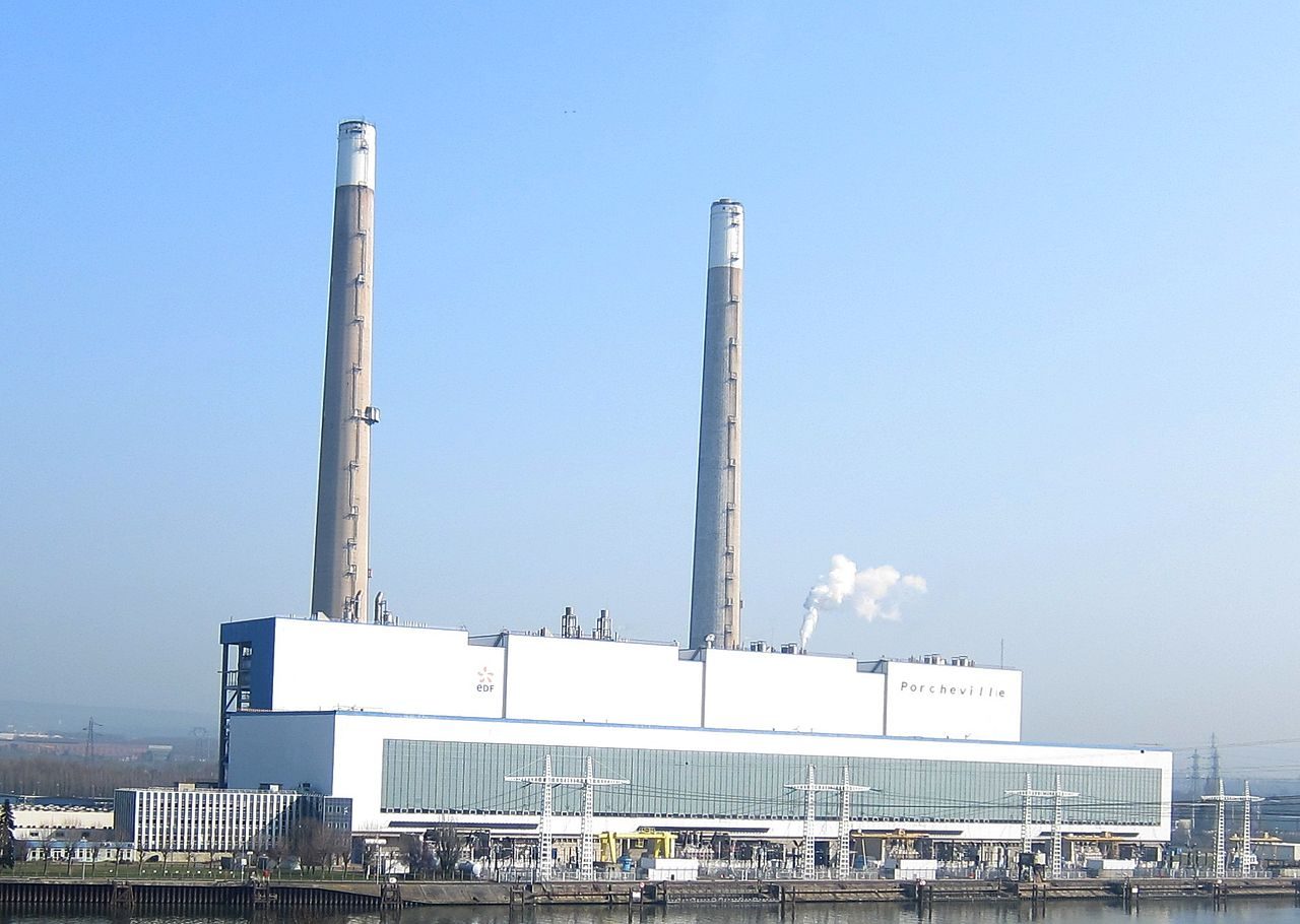
Figure 9.27:The Porcheville power plant, running on coal until 1987, then on oil until 2017, when it closed down. It mainly served peak demands.

What hourly steam flow rate is required in the circuit in order to achieve a net power of $60 MW$ ?

Exercise 9.2

Implementation of a reheating process The Porcheville power plant described in Problem 9.1 is modified to accommodate a series of reheating tubes. The water expansion is stopped at 18 bar in the turbines, and the steam is brought back to the maximum temperature of the cycle (that is, $545^{\circ}C)$ . The power plant is fueled by heavy fuel oil known as “ulsd”, with a density of $1050 kg m^{-3}$ and a heat of combustion of $40.2 MJ kg^{-1}$ . The air used for combustion enters the boiler at a temperature of $15^{\circ}C$ and a pressure of 1 bar. It is heated to a temperature of $820^{\circ}C$ at constant pressure through combustion, before passing around the water pipes. When it leaves the boiler, its temperature is $180^{\circ}C$ . 1. What is the new thermal efficiency of the power plant? 2. What is its new specific steam consumption? 3. What air flow rate must be admitted to the boiler in order to maintain a net power of $60 MW$ ? 4. What is the boiler efficiency? 5. What is the hourly volumetric flow rate of fuel? 6. An engineer proposes to pass the intake air duct through the exhaust gases (without mixing them) to increase its temperature before combustion. Do you think this is a good idea?

Answer

$h_{\mathrm{D}2}= 2960.8 kJ kg^{-1}, h_{\mathrm{E}2}= 3570.3 kJ kg^{-1}$ , $h_{\mathrm{F}}= 2642.7 kJ kg^{-1}$ , thus the efficiency reaches $\eta _{\mathrm{thermal} 2}= 36.31 \%$ (+1 point, already a significant improvement); 2) ssc = $2.576 kg/(kW h) (-18 \%$ , good work); 3) In the boiler, the heat rejected by the air is gained by the water: $\dot{m}_{\mathrm{air}}= \frac{-Q\dot{} _{\mathrm{water}}}{c_{p}\Delta T} = \frac{W_{\mathrm{net}}}{\eta _{\mathrm{thermal}}} c_{p}(T_{\mathrm{air}}1_{3}-T_{\mathrm{air} 2}) = 256.9 kg s^{-1}.4) \eta _{\mathrm{boiler}}=5)\dot{V}_{\mathrm{fuel}}3893 imp gal/h$ ; $=^{Q_{\mathrm{received} \mathrm{by} \mathrm{the} \mathrm{air}}}= 79.5 \%$ ; $_{\rho _{\mathrm{fuel}}c_{\mathrm{fuel}}\eta _{\mathrm{boiler}}}= 17.7 m^{3}h^{-1}=$
It is an excellent idea. In this way, we reduce the heat carried away by the exhaust gases at the boiler outlet, immediately increasing $\eta _{\mathrm{boiler}}$ .

Exercise 9.3

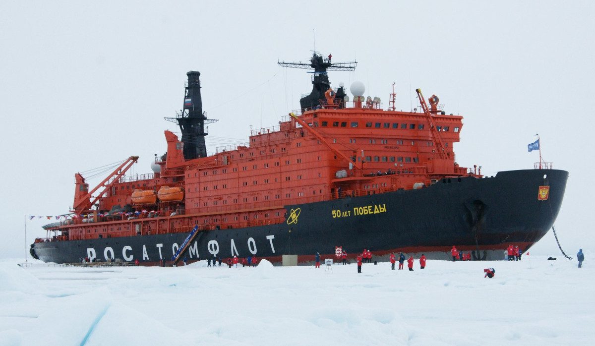
Cycle with regeneration In a polar icebreaker ship (figure 9.28), the propellers are driven by a steam system, itself powered by a nuclear reactor. The cycle is based on a superheated Rankine cycle between pressures of 30 and 0.5 bar. The steam, heated by a secondary pressurized water system that passes through the reactor, reaches $310^{\circ}C (590 ^{\circ} F)$ . For the sake of not overloading this problem, we consider that the turbine is isentropic and perfectly insulated. 1. What is the thermal efficiency of the power plant? 2. We define the specific steam consumption as the inverse of the net power of the power plant: it is the mass of steam that has passed through the turbine when the power plant has generated $1 kWh$ of work. What is the specific consumption of the power plant? Photo CC-by-sa by Commons User:Kiselev d An engineer proposes to modify the cycle and make it regenerative by extracting steam from the turbine to insert it into the compression circuit. S/he suggests separating the compression into two stages, one from 0.5 bar to 6 bar, and the second from 6 bar to 30 bar; and then inserting the extracted steam into the feedwater between the two pumps. The steam extraction rate is such that the water at the outlet of the mixer is exactly at the saturation point. 1. Make a sketch of the proposed setup (that is, the physical circuit followed by the steam). 2. Draw the cycle qualitatively (that is, without showing numerical values) on a temperature-entropy diagram, showing the saturation curve. 3. What percentage of the turbine steam flow rate would need to be extracted at 6 bar in order to heat the water to saturation between the two pumps? 4. Does the shaft power increase or decrease, and by how much? 5. Does the efficiency of the power plant increase or decrease, and by how much?

Answer

The 50 Let Podeby actually operates between $29 a$ nd 0.75 bar, but these values that are not tabulated in the steam tables for this book. 1) Using the diagram from figures 9.14 and 9.15 on page 256, $h_{\mathrm{A}}= 340.5 kJ kg^{-1}, h_{\mathrm{B}}= 343.54 kJ kg^{-1}$ , $h_{\mathrm{D}}= 3017.4 kJ kg^{-1}, h_{\mathrm{E}}= 2284.5 kJ kg^{-1}$ , thus $\eta _{\mathrm{thermal}}= 27.294 \%$ ; 2) ssc $= 4.93 kg/(kW h)$ ; 3) See figure 9.20 p. 259; 4) See figure 9.21 p. 259; 5) $h_{\mathrm{bleed}}= 2673.9 kJ kg^{-1}, h_{\mathrm{pre-mix}}= 341.1 kJ kg^{-1}$ , $h_{\mathrm{post-mix}}= 670.4 kJ kg^{-1}$ : thus the proportion needed to saturate the water after mixing is $z = 14.1 \%$ ; 6) $w_{\mathrm{net} 2}= -674.87 kJ kg^{-1}(-9.2 \%$ : a tragedy!); 7) $q_{\mathrm{boiler}}= 2344.4 kJ kg^{-1}$ , thus $\eta _{\mathrm{thermal} 2}= 28.786 \% (+1.49 pt$ : is it really desirable in this application?).

The 50 Let Podeby, a 25,000-ton nuclear-turbo-electric powered icebreaker (two reactors of , three engines of . Its construction started in — Figure 9.28:The *50 Let Podeby*, a 25,000-ton nuclear-turbo-electric powered icebreaker (two reactors of $171 MW_{\mathrm{heat}}$ , three engines of $17.6 MW_{\mathrm{mech}.})$ . Its construction started in 1989 but it only entered service in 2007.