4. The Ideal Gas - Engineering Thermodynamics

4. The Ideal Gas¶

The Ideal Gas

The Improbable Thermometer of Scholar Clapeyron

Introduction¶

In chapters 2 and 3 we learned to quantify energy transfers — but we can only do so when we know the values of $u$ or $h$ , which are quantities that are impossible to measure directly in practice.

This chapter 4 (the ideal gas) aims to answer two questions:

• How can we describe the behavior of air when it is heated or compressed?

• How can we predict the values of $u$ and $h$ when using air?

This chapter is incompatible with chapter 5 (liquids and vapors), where we will have to forget everything learned here.

4.1 Definition¶

4.1.1 The manometer as a thermometer¶

Let us start with the most important point:

The ideal gas model defines by itself a temperature scale. It is proposed to measure the absolute temperature $T$ very simply with a manometer, stating that it is directly proportional to the pressure $p$ and inversely proportional to the density $\rho$ .

We can thus say that the ideal gas does not describe the reality of things, that it is not a physical principle, but only a simplified model of gas behavior. Its range of validity is limited and fuzzy.

4.1.2 Definition: the equation of state¶

We will call ideal gas a fluid in the gaseous state whose product of pressure and volume, $pv$ , remains proportional to its temperature. The proportionality constant is called the gas constant, denoted as $R$ ; it depends on the nature of the gas.

pv = RT

(4/1)

by definition for an ideal gas, where $p$ is the pressure $(Pa)$ , $v$ is the specific volume $(m^{3}kg^{-1})$ , $T$ is the temperature $(K)$ , and $R$ is the gas constant of the considered gas $(J K^{-1}kg^{-1})$ .

Equation 4/1 is called the equation of state of ideal gases. It can also be expressed in terms of mass:

pV = mRT

(4/2)

where $V$ is the volume $(m^{3})$ , and $m$ is the mass of the gas considered $(kg)$ .

It is also possible to express Equation 4/2 in terms of the amount of substance in moles.^[1] Because it is inseparable from the concept of absolute temperature, it took 150 years for this equation to take its final form: the one given by Émile Clapeyron in 1834 [5].

Example 4.1

A mass of $2 kg$ of gas with a constant $R = 100 J K^{-1}kg^{-1}$ is contained in a reservoir of $200 L (52.83 US gal)$ at a pressure of $3 bar (43.51 psi)$ . What is its temperature?

We start from Equation 4/2 to express the temperature: $T = \frac{p V}{m R} = \frac{3\times 10^{5}\times 0.2}{2\times 100} = 300 K = 26.85^{\circ}C = 80.33 ^{\circ} F$ .

Admirable Émile! The simplicity of this calculation will be missed in the next chapter.

The only thorn in this equation concerns the units, which must be properly converted to SI: $200 L = 0.2 m^{3}$ and $3 bar = 3 \times 10^{5}Pa$ . The temperature is always in kelvins.

Example 4.2

Atmospheric air can be modeled as an ideal gas with $R_{\mathrm{air}}= 287 J kg^{-1}K^{-1}$ . Under ambient conditions $(1 bar, 20^{\circ}C$ , that is, $14.5 psi$ and $68 ^{\circ} F)$ , what are the specific volume and the density of the atmosphere?

We start from Equation 4/1 to express the specific volume: $v = \frac{R T}{p} = \frac{287\times (20+273.15)}{1\times 10^{5}} = 0.841 m^{3}kg^{-1}$ . The density then follows simply: $\rho = \frac{1}{v} = 1.189 kg m^{-3}$ .

Once again, forgetting to convert the temperature units to kelvins would be fatal (try using $0^{\circ}C$ or $0 ^{\circ} F$ ).

In one cubic meter $(220 gal imp)$ , we have only $1.2 kg (2.6 lb)$ of air. This is very little, especially when compared to liquid water $(1000 kg$ for the same volume). Air machines typically operate with large volumetric flow rates.

4.1.3 What does an ideal gas represent?¶

The ideal gas is the simplest model one can imagine to represent the behavior of a gas.

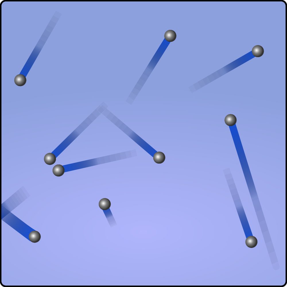
According to this model, molecules behave like spheres bouncing off each other (figure 4.1). One can imagine a large number of very small billiard balls in chaotic motion, colliding and bouncing off each other without attracting one another or dissipating their energy through friction.

Figure 4.1:An ideal gas can be visualized as a set of balls in random motion. They collide without friction and without mutual attraction. The speed of each ball changes with each collision.

Diagram CC-by-sa by Commons User:Sharayanan & Olivier Cleynen

In this chaos, temperature is a measure of the kinetic energy of the molecules. It is quantified by measuring the time-averaged force resulting from the impact of the molecules on a wall of the container – that is, with pressure. With this model, we can propose a temperature scale such that $T \propto p$ .

The fewer molecules impacting the surface, and the more forcefully they must impact it in order to generate a given pressure. Thus, when the density $\rho$ decreases at a given pressure, it means that the temperature is increasing: we can also propose $T \propto \frac{1}{\rho}$ .

If these two proposals are combined into a single equation, we obtain a simple model to quantify temperature: $T \propto pv$ .

4.1.4 What does an ideal gas** not **represent?¶

The behavior of molecules when they are close to each other is actually very complex, since the attractive forces then play a decisive role. The influence of these forces is all the more significant when the molecules are slow and structurally complex (the interaction between two hydrocarbon molecules, for example, is more difficult to model than the interaction between two helium molecules).

The macroscopic consequences of these interactions, and the conditions under which they should no longer be neglected, are addressed in chapter 5 (liquids and vapors).

For now, we will remember that the ideal gas model works better:

• When molecules collide at high speed, that is, when the gas temperature is high;

• When the average space between molecules is large, that is, when the specific volume of the gas is large.

These conditions ensure that the attractive forces between molecules can only play a minor role in the overall behavior of the gas. They are met for air in the vast majority of engineering applications. We will use the value

R_{\mathrm{air}}= 287 J kg^{-1}K^{-1} for pure air in our machines.

(1)

4.1.5 Model limitations¶

It will not take long for the student to find the limits of Equation 4/2, which indicates that a non-zero mass of ideal gas occupies zero volume at zero temperature. Strictly speaking, the ideal gas cannot exist – the mathematical model loses its meaning at very low temperatures since it does not take into account the volume of the molecules themselves.

Several other equations of state can be used to better match real gases over a wider range of properties.

Thus, the Van der Waals equation, proposed as early as the late 18th century, suggests:

(p + \frac{a}{v^{2}})(v - b) = RT

(4/3)

where $a$ and $b$ are two constants.

This equation has the advantage of taking into account two factors ignored in the equation of state 4/1: the attractive force between molecules (the term $a/v^{2}$ , which becomes part of the pressure expression) and the volume occupied by the molecules themselves (the term $b$ which is subtracted from the available volume).

Despite the difficulties inherent in quantifying the terms $a$ and $b$ , these modifications have significantly extended the range of application of equations of state. They earned their author, Johannes Diderik Van der Waals, the Nobel Prize in Physics in 1910.

Building mathematical models to describe the state of real gases is an important research area in fluid mechanics. The curious student can refer to equations of state such as the Beattie-Bridgeman, Benedict-Webb-Rubin, or the Strobridge models, in order get an overview of their increasing complexity. As for us, we will stick to equation 4/1.

4.2 Properties of Ideal Gases¶

4.2.1 Two important thermal capacities¶

We have already discussed the concept of thermal capacity in the first chapter (1/16). It is defined as the amount of heat required to increase the temperature of one kilogram of the substance by one Kelvin (or one degree Celsius, since these temperature differences are equal). Thus, we have:

c = \frac{\mathrm{δ}q}{dT}

(4/4)

where $c$ is the specific thermal capacity $(J K^{-1}kg^{-1})$ , δ $q$ the (specific) infinitesimal heat transfer $(J kg^{-1})$ , and $dT$ the produced infinitesimal change in temperature $(K)$ .

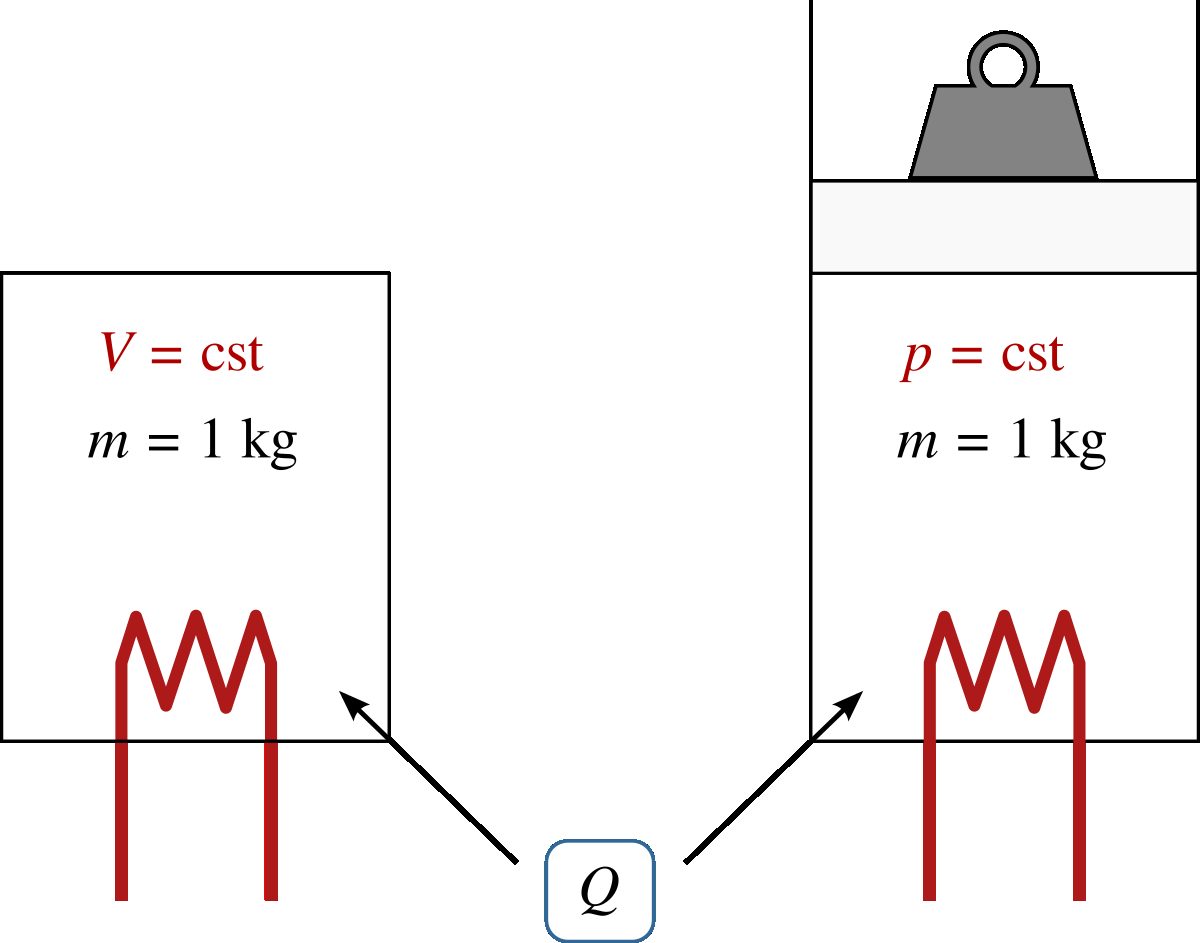
Since the temperature of a gas also varies when work is done on it or by it, there are an infinite number of different ways to change its temperature by one degree, by combining heat and work (figure 4.2). Each of these requires a unique amount of heat; thus, there are infinitely many thermal capacities associated with it.

Two identical quantities of gas receive the same amount of heat $Q$. The temperature increase will be lower on the right due to the work done on the piston. — Figure 4.2:Two identical quantities of gas receive the same amount of heat $Q$ . The temperature increase will be lower on the right due to the work done on the piston.

Diagram CC-0

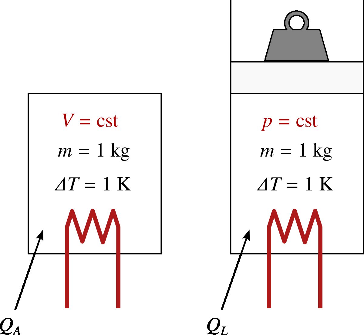
Among these, two particular values (figure 4.3) serve as references for describing the behavior of an ideal gas:

the thermal capacity at constant volume: $c_{v}$ ,

the thermal capacity at constant pressure: $c_{p}$ .

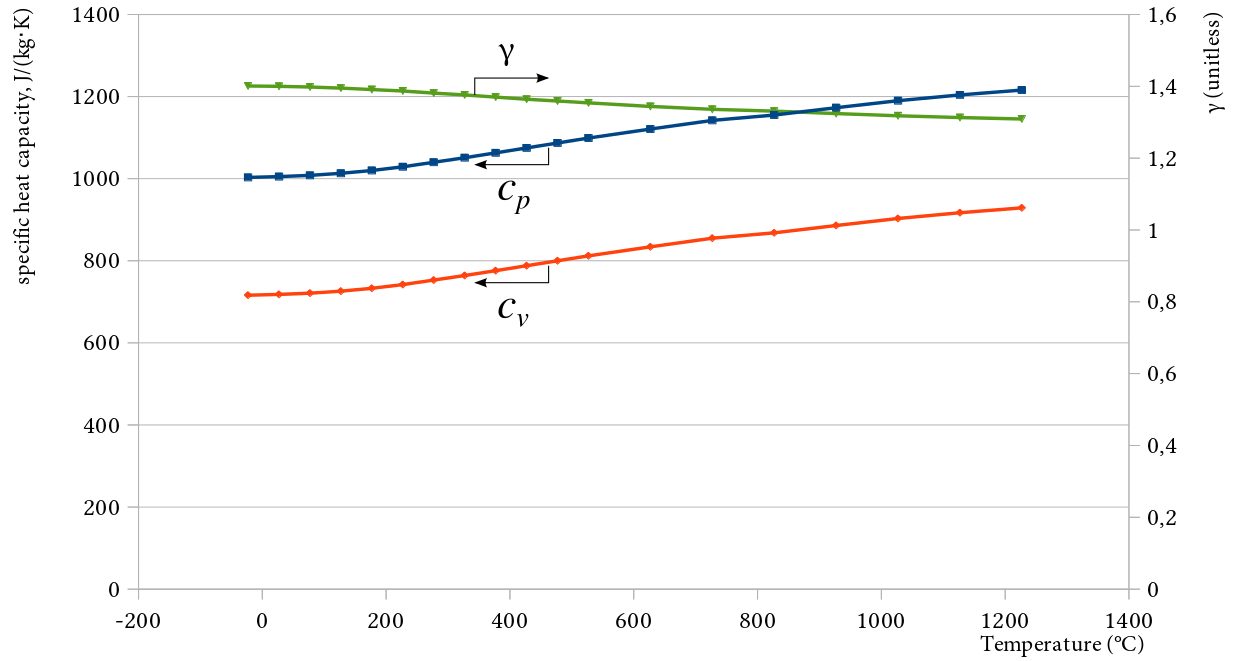
These two quantities are properties (or state quantities, see Appendix A4 p. 316), and we will soon use them to quantify energy in gases. In an ideal gas, $c_{v}$ and $c_{p}$ are independent of temperature. In real gases, these capacities vary with temperature (figure 4.4), but for most hand-written engineering applications, it is reasonable to use average values. For air, we will take $c_{v (\mathrm{air})}= 718 J kg^{-1}K^{-1}$ and $c_{p (\mathrm{air})}= 1005 J kg^{-1}K^{-1}$ .

Definitions of heat capacities. On the left, the volume is fixed and the specific thermal capacity will be $c_{v}$. On the right, the pressure is constant and the capacity will be $c_{p}$. — Figure 4.3:Definitions of heat capacities. On the left, the volume is fixed and the specific thermal capacity will be $c_{v}$ . On the right, the pressure is constant and the capacity will be $c_{p}$ .

Diagram CC-0

Figure 4.4:Specific thermal capacity of air as a function of temperature. There is a noticeable change in values in the temperature range used in engineering, which we will neglect in the scope of this book.

Data from NBS Circular 564 “Tables of Thermal Properties of Gases” (1955) up to $1000 K$ , calculated

according to the model of B. G. Kyle in “Chemical and Process Thermodynamics” (1984) above $1000 K$ , and published by Israel Urieli

4.2.2 Difference of thermal capacities¶

The large number of equations we are discussing makes this short section 4.2.2 useful, but not essential. For the engineer, its only interest is to simplify the writing of the equations in the section that comes after it.

Let us observe the amounts of energy involved in the experiment described in figure 4.3. We supply each body with a different amount of heat to achieve the same temperature change. The difference between the two required amounts of heat comes from the fact that the gas at constant pressure (on the right) has done work during the process.

What is the difference between the thermal capacities of each? In both cases, we have $q_{1\rightarrow 2}+ w_{1\rightarrow 2}= \Delta u$ (2/2). For body A on the left, since no work is done and the process is at constant volume, we can write:

q_{\mathrm{A}}= c_{v}\Delta T

(4/5)

\Delta u = q_{\mathrm{A}}

(2)

For body B on the right, with constant pressure $p_{\mathrm{cst}.}$ , we can write:

q_{\mathrm{B}}= c_{p}\Delta T

(4/6)

\Delta u = q_{\mathrm{B}}+ (-p_{\mathrm{cst}.}\Delta v)

(3)

By combining the two systems 4/5 and 4/6, we obtain

c_{v}\Delta T = c_{p}\Delta T - p_{\mathrm{cst}.}\Delta v

(4/7)

This simply states that the difference between the two amounts of heat supplied to the gas is found in the work done by the gas on the right. (To be truly rigorous, in order to assert that $\Delta u_{A}$ and $\Delta u_{B}$ are equal, we would need to wait for equation 4/11 which comes in the next section.)

A little algebra leads to:

(c_{p}- c_{v})\Delta T = p_{\mathrm{cst}.}\Delta v

(4)

(c_{p}- c_{v}) = \frac{pv_{2}- pv_{1}}{\Delta T} = \frac{RT_{2}- RT_{1}}{\Delta T} = \frac{R \Delta T}{\Delta T}

(5)

c_{p}- c_{v}= R

(4/8)

This expression only serves to simplify equation 4/13 that we will write below.

4.2.3 Ratio of thermal capacities¶

The ratio of thermal capacities at constant pressure and constant volume is named $\gamma$ . Thus:

\gamma \equiv \frac{c_{p}}{c_{v}}

(4/9)

By returning to figure 4.3 it quickly appears that $c_{p}$ must be greater than $c_{v}$ ; thus $\gamma$ is always greater than 1. We take $\gamma _{\mathrm{air}}= 1.4$ .

4.3 Energy and Temperature¶

4.3.1 Historical context¶

The first research undertakings aimed at exploring the concept of temperature took place at the very beginning of the 19th century. The scientific community was then very interested in gases – it was noticed that there are two ways to increase their temperature: by heating them, but also by compressing them.

Frenchman Joseph Louis Gay-Lussac sought to understand why the temperature of a gas drops when it expands (he actually sought, according to the concepts of the time, to identify the source of the caloric and the reasons why it flows). He thus endeavored to produce gas expansions that were as simple as possible, and to measure the temperature. Thirty years later, the Englishman James Prescott Joule resumed and deepened these experiments, but this time, by quantifying heat as work equivalence. These experiments with gas balloons and thermometers are anything but spectacular – but they would play a pivotal role in thermodynamics, because they allowed for the first time to distinguish heat, work, energy, and temperature. Joule’s meticulous work lead to the first formal expression of the first law of thermodynamics, and to the end of the caloric theory according to which heat was a very low-density and invisible fluid. Our modern unit for energy is named after him as a tribute to these results.

4.3.2 Joule’s law¶

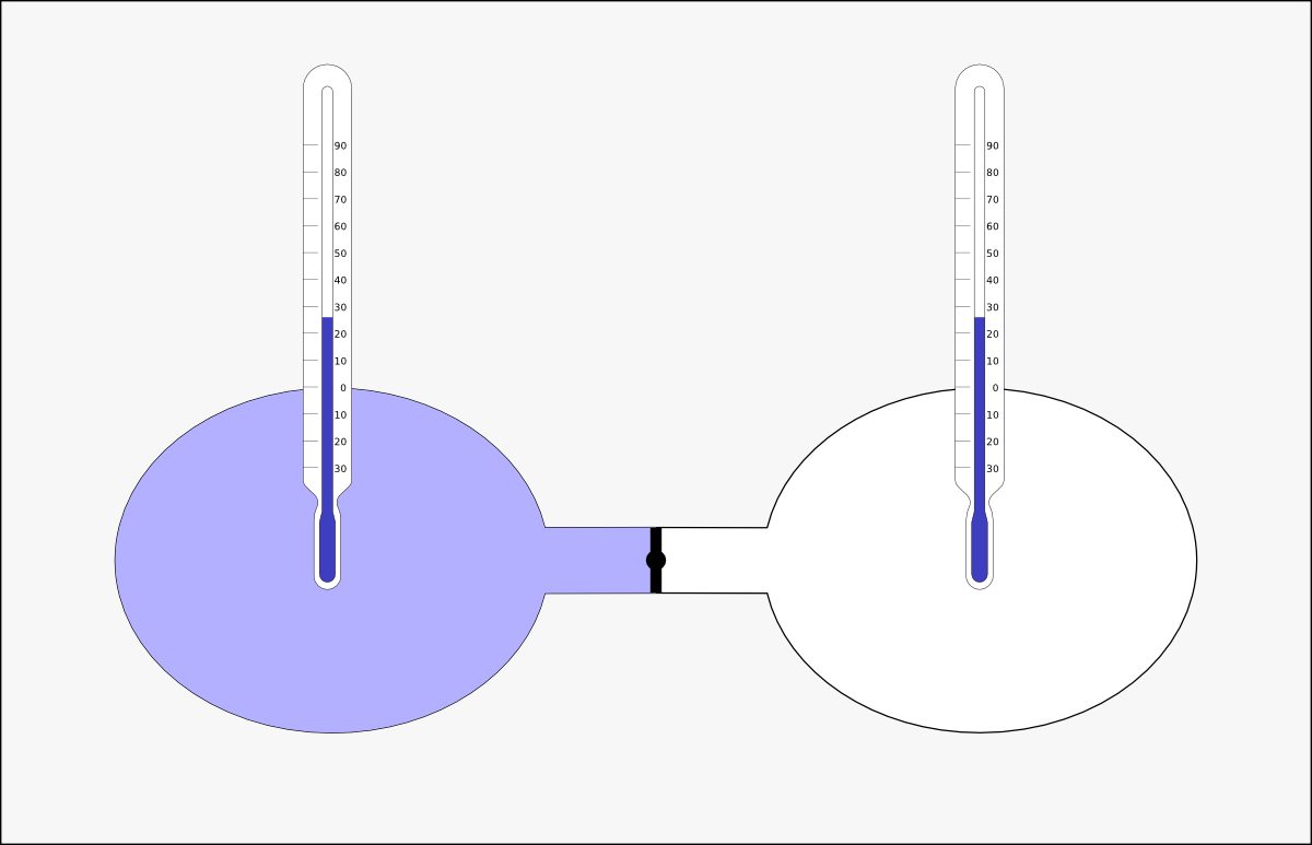
In their most remarkable experiment, Joule and Gay-Lussac were seeking to vary the pressure and volume of a gas without transferring heat or work to it. For this, they let a compressed gas in a container expand into a second, empty container (figure 4.5). The work done was zero, since no surface had been moved – the process was entirely irreversible. The temperature was measured and... nothing happened! Joule and Gay-Lussac measured neither heat transfer nor temperature variation.

Figure 4.5:The expansion of Joule and Gay-Lussac. A gas is initially trapped in a reservoir on the left; it is allowed to expand by opening the valve (in the center) which separates it from a completely empty reservoir on the right. Joule and Gay-Lussac are interested in the temperature changes measured in each reservoir. The closer the gas properties resemble the behavior of ideal gases model (§4.1.4), the smaller the temperature changes they measure, becoming undetectable for some simple gases at high temperatures.

Diagram CC-0 Olivier Cleynen

Joule carried out a multitude of different experiments during which he observed that regardless of the supplied work, the relationship between internal energy (which varies only with work and heat) and temperature remained essentially the same – and he suggested that for an ideal gas, it always remains identical.

This postulate is known as Joule’s law and is posited as true for any ideal gas. It can be summarized as follows:

The temperature of an ideal gas only varies with its internal energy.

Mathematically, we can write it as:

u = f(T)

(4/10)

The function $f$ can be evaluated with an experiment in which the change of $u$ is quantified. For example, during a process at constant volume $q = \Delta u$ and $q = c_{v}\Delta T$ . We can thus assert that the function $f$ is a simple proportional relation. With the internal energy arbitrarily set to zero at zero temperature $(u = 0 J kg^{-1}$ when $T = 0 K)$ , we obtain:

u = c_{v}T

(4/11)

for any ideal gas, regardless of the process (reversible or not), where $u$ is the specific internal energy $(J kg^{-1})$ ; $T$ is the temperature $(K)$ ;

and $c_{v}$ is the specific thermal capacity at constant volume $(J kg^{-1}K^{-1})$ .

For a mass $m$ of ideal gas, we have of course:

U = m c_{v}T

(4/12)

As long as our fluid behaves as an ideal gas, this relation 4/11 remains true. It works for any process, reversible or not, and regardless of volume, pressure, or temperature constraints.

On the other hand, it should be noted that this equation 4/11, which results from Joule’s law, does not work all for liquids and vapors. For example, we can add energy to a mass of boiling water without its temperature increasing. We will study liquids and vapors in chapter 5.

Example 4.3

The specific thermal capacity at constant volume for air is measured at $c_{v (\mathrm{air})}= 718 J kg^{-1}K^{-1}$ . We take a mass of $0.5 kg$ of air at $20^{\circ}C$ and transfer $+15 kJ$ as heat and $-10 kJ$ as work. What is its final temperature?

We know that the energy has varied with the transfers: $\Delta U = W_{\mathrm{A}\rightarrow \mathrm{B}}+ Q_{\mathrm{A}\rightarrow \mathrm{B}}= m c_{v}\Delta T$ . Thus, the temperature has varied proportionally: $T_{\mathrm{B}}= T_{\mathrm{A}}+ \frac{\Delta U}{m c_{v}} = T_{\mathrm{A}}+ \frac{W_{\mathrm{A}\rightarrow \mathrm{B}}+ Q_{\mathrm{A}\rightarrow \mathrm{B}}}{m c_{v}}= 20 + \frac{-10\times 10^{3}+(+15\times 10^{3})}{0.5\times 718}= 33.92^{\circ}C$ .

Good old James! We just only need to quantify the energy changes to know the temperature, and vice versa.

Here the temperatures in degrees Celsius are only added and a conversion to kelvins would not have changed the result. In case of doubt, it is better not to take this shortcut.

4.3.3 Enthalpy of an ideal gas¶

Because we have just linked the internal energy $u$ to the temperature, and because and the product $pv$ also depends on the temperature, we can now easily express the enthalpy $h$ of an ideal gas in terms of temperature only.

Indeed, we have $h \equiv u + pv$ (3/12); with a quick insertion of equations 4/1 and 4/11 we can write, for any ideal gas:

h = u + pv = c_{v}T + RT = (c_{v}+ R) T

(4/13)

Using the equation 4/8 that we developed earlier, we can simplify this expression to obtain:

h = c_{p}T

(4/14)

For any ideal gas, regardless of the process (reversible or not), where $h$ is the specific enthalpy $(J kg^{-1})$ ; $T$ is the temperature $(K)$ ; and $c_{p}$ is the specific thermal capacity at constant pressure $(J kg^{-1}K^{-1})$ .

Example 4.4

The specific thermal capacity at constant pressure for air is measured at $c_{p (\mathrm{air})}= 1005 J kg^{-1}K^{-1}$ . A flow rate of $2 kg s^{-1}$ of air passes through a compressor, where its temperature increases by $150^{\circ}C$ . What is the power supplied by the compressor to the air?

We know that the change in energy is directly proportional to the change in temperature. Using equations 3/14 and 4/14, we obtain: $\dot{W}_{\mathrm{A}\rightarrow \mathrm{B}}+\dot{Q}_{\mathrm{A}\rightarrow \mathrm{B}}=\dot{m} \Delta h =\dot{m} c_{p}\Delta T = 2 \times 1005 \times (+150) = +301.5 kW$ .

With an ideal gas, a simple thermometer is enough to quantify energy…

…but not to differentiate work and heat. Here we cannot separate $\dot{W}_{\mathrm{A}\rightarrow \mathrm{B}}$ from $\dot{Q}_{\mathrm{A}\rightarrow \mathrm{B}}$ . We also cannot predict the state of the gas at the outlet, that is its pressure $p$ and specific volume $v$ (only their product). For this, a precise description of what happens between the inlet and the outlet would be needed.

4.3.4 Interlude: what to remember so far¶

The ideal gas is a model for quantifying the temperature of a gas. According to this model, the three main forms of energy we have used so far — internal energy $u$ , enthalpy $h$ , and the term $pv$ — are directly proportional to the temperature $T$ :

u = c_{v}T \qquad h = c_{p}T \qquad pv = RT

(6)

If we measure the absolute temperature of a gas, then we can immediately quantify these three forms of energy.

4.4 Elementary Reversible Processes¶

Here we intend to calculate the properties of an ideal gas, as well as the energy transfers involved, when it is compressed or expanded under completely arbitrary constraints of volume, pressure, or temperature.

4.4.1 What is this chapter section for?¶

The gas processes we study here are very hypothetical and not necessarily exciting, but they deserve the attention of the student for two reasons:

The behavior of gases is inherently complex, even when we use the ideal gas model. These elementary processes serve as small exercises for us, to help us learn step by step;
These elementary processes are conceptual tools that we will later assemble, first to quantify the theoretical limits of machines (in chapter 7), and then to describe the behavior of gases inside real machines (in chapter 10).

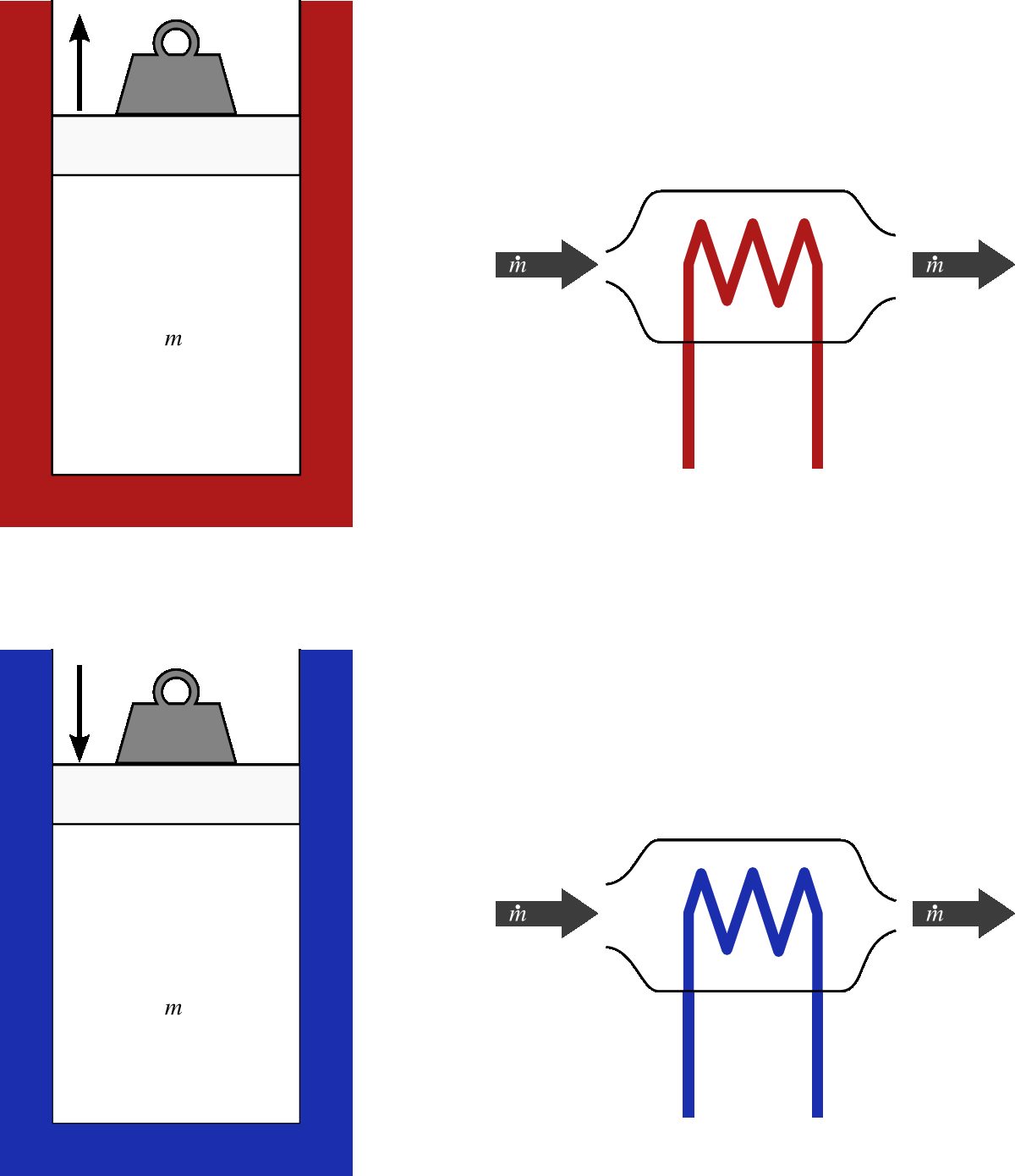
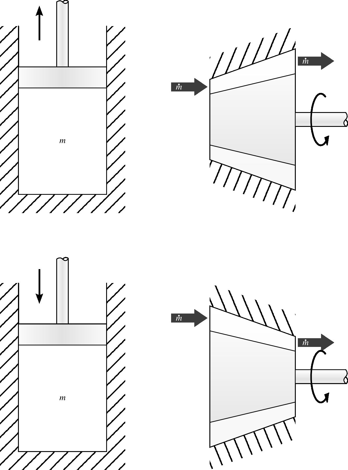
4.4.2 Processes at constant pressure¶

It is possible to heat or cool a gas while maintaining its pressure constant (figure 4.6). A process at constant pressure is called isobaric. In order to generate such a process, we can:

• with a closed system, heat or cool the gas while maintaining a constant force on the walls;

• with an open system, heat or cool the gas by simply letting it flow in a duct, without any moving parts. This is the case, for example, in the combustion chamber of a jet engine.

When the pressure is constant, the properties of the gas vary according to the relation

\frac{T}{v} = \mathrm{constant}

(4/15)

Figure 4.6:A constant-pressure (isobaric) process undergone by an ideal gas. In a closed system (left), the piston exerts a constant force throughout the process. In an open system (right), no work is done.

Diagram CC-0 Olivier Cleynen

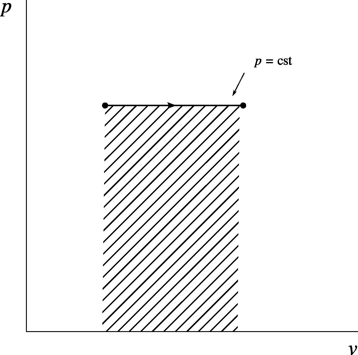
Figure 4.7:Heating at constant pressure of an ideal gas, represented on a pressure-volume diagram.

Diagram CC-0 Olivier Cleynen

In a closed system, we have $q_{1\rightarrow 2}+ w_{1\rightarrow 2}= \Delta u$ (2/2) and, if the process is reversible, heat and work can be easily related to the temperature:

\begin{aligned} w_{1\rightarrow 2}&= -\int_{1}^{2} pdv = -p_{\mathrm{cst}.}\int_{1}^{2} dv = -p_{\mathrm{cst}.}\Delta v \end{aligned}

(7)

w_{1\rightarrow 2}= -R \Delta T

(4/16)

during a reversible process at constant pressure $p_{\mathrm{cst}.}$ , in a closed system.

We notice that the work is of opposite sign to the change in temperature.

Heat can be easily quantified:

q_{1\rightarrow 2}= \Delta u - w_{1\rightarrow 2}= \Delta u + p_{\mathrm{cst}.}\Delta v = \Delta h

(8)

q_{1\rightarrow 2}= c_{p}\Delta T

(4/17)

during a reversible process at constant pressure, in a closed system.

When the process takes place in an open system, we have $q_{1\rightarrow 2}+ w_{1\rightarrow 2}= \Delta h$ (3/15), and, if the process is reversible, heat and work can be easily quantified:

\begin{aligned} w_{1\rightarrow 2}&= \int_{1}^{2} vdp \end{aligned}

(9)

w_{1\rightarrow 2}= 0

(4/18)

during a reversible process at constant pressure, in an open system.

The work is of course zero, since there are no moving parts present to mechanically extract energy from the gas.

Heat is then responsible for the entire change in temperature:

q_{1\rightarrow 2}= \Delta h - w_{1\rightarrow 2}= \Delta h

(10)

q_{1\rightarrow 2}= c_{p}\Delta T

(4/19)

during a reversible process at constant pressure, in an open system.

Example 4.5

For air, we have $c_{p (\mathrm{air})}= 1005 J kg^{-1}K^{-1}, c_{v (\mathrm{air})}= 718 J kg^{-1}K^{-1}, R_{\mathrm{air}}= 287 J kg^{-1}K^{-1}$ . How much energy is needed to heat the air in a $30 m^{2} (322.9 ft^{2})$ apartment from $10^{\circ}C$ to $20^{\circ}C (50 ^{\circ} F$ to $68 ^{\circ} F)$ ?

The heating will likely take place at constant pressure (unless the apartment is hermetically sealed, the pressure will be atmospheric everywhere and the air will “leak” under the doors). We assume a pressure of 1 bar and a ceiling height of $2.5 m$ . We use a closed system encompassing all the heated air.

We have a volume of $75 m^{3}$ , which leads to the total mass of air as $m_{\mathrm{A}}= \frac{p_{\mathrm{A}}V_{\mathrm{A}}}{R T_{\mathrm{A}}} = \frac{1\times 10^{5}\times 75}{287\times (10+273.15)}= 92.29\,\mathrm{kg} = 203.5\,\mathrm{lb}$ . The heat required to heat this amount of air at constant pressure can be quantified with equation 4/17: $Q_{\mathrm{A}\rightarrow \mathrm{B}}= m c_{p}\Delta T = 93.29 \times 1005 \times (20 - 10) = +9.28 \times 10^{5}J = +928 kJ$ .

This result represents the final net heat transfer to the air (after losses to walls and windows, as well as transfers that compensate for them).

Conversely, cooling would cause outside air to come in, which would need to be taken into account in the mass calculation.

4.4.3 Processes at constant volume¶

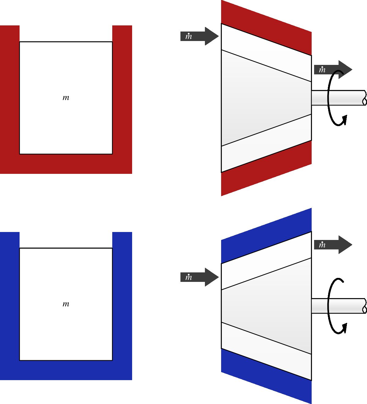
It is possible to heat or cool a gas while maintaining its volume constant (figure 4.8). A process at constant volume is called isochoric.

• With a closed system, we can heat or cool a gas in a fixed and closed reservoir. This is the case, for example, during the combustion phase in a gasoline engine.

• With an open system, the manipulation is more complex. When heating the gas, we must compress it, in order to prevent its volume from increasing; conversely, while cooling it, we must expand it so as to prevent its volume from decreasing. This manipulation has no common practical application.

When the specific volume of a perfect gas is constant, its properties vary according to the relation

\frac{T}{p} = \mathrm{constant}

(4/20)

In a closed system, we have $q_{1\rightarrow 2}+w_{1\rightarrow 2}= \Delta u$ and, if the process is reversible, heat and work can be easily related to temperature.

Since the volume does not change, the work is of course zero:

\begin{aligned} w_{1\rightarrow 2}&= -\int_{1}^{2} pdv = 0 \end{aligned}

(11)

w_{1\rightarrow 2}= 0

(4/21)

during a reversible process at constant volume, in a closed system.

Figure 4.8:A constant-volume (isochoric) process undergone by an ideal gas. In a closed system (left), the volume is fixed and no work is done. In an open system (right), the gas must be compressed while heating and expanded while cooling, to maintain the specific volume constant.

Diagram CC-0 Olivier Cleynen

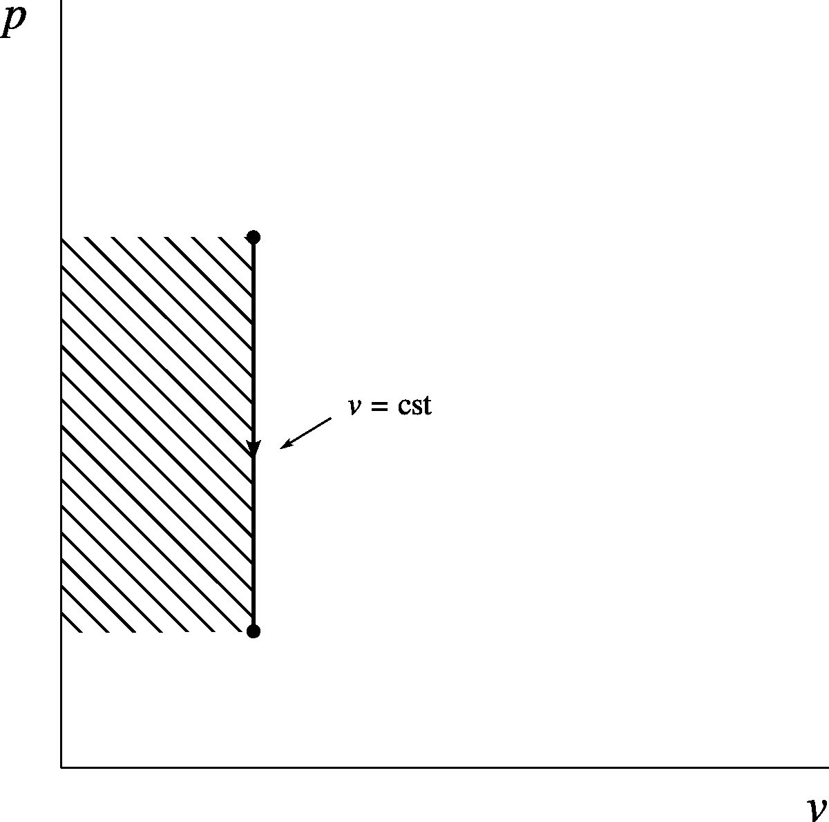
Figure 4.9:Cooling of an ideal gas at constant volume, represented on a pressure-volume diagram.

Diagram CC-0 Olivier Cleynen

The heat transfer can be easily quantified:

q_{1\rightarrow 2}= \Delta u - w_{1\rightarrow 2}= \Delta u

(12)

q_{1\rightarrow 2}= c_{v}\Delta T

(4/22)

during a reversible process at constant volume, in a closed system.

When the process occurs in an open system, we have $q_{1\rightarrow 2}+ w_{1\rightarrow 2}= \Delta h$ and, if the process is reversible, heat and work can be quantified, although with a little more difficulty:

w_{1\rightarrow 2}= \int _{1}^{2}vdp = v_{\mathrm{cst}.}\int _{1}^{2}dp = v_{\mathrm{cst}.}\int _{1}^{2} \frac{R}{v_{\mathrm{cst}.}} dT = R\int _{1}^{2}dT

(13)

w_{1\rightarrow 2}= R \Delta T

(4/23)

during a reversible process at constant volume, in an open system.

One can then easily quantify the heat to be supplied:

q_{1\rightarrow 2}= \Delta h - w_{1\rightarrow 2}= c_{p}\Delta T - R \Delta T

(14)

q_{1\rightarrow 2}= c_{v}\Delta T

(4/24)

during a reversible process at constant volume, in an open system.

Example 4.6

For air, we measure $c_{p (\mathrm{air})}= 1005 J kg^{-1}K^{-1}, c_{v (\mathrm{air})}= 718 J kg^{-1}K^{-1}$ , $R_{\mathrm{air}}= 287 J kg^{-1}K^{-1}$ . In a cylinder of a gasoline engine, air is at a pressure of $17 bar (246.6 psi)$ with a density of $9.4 kg m^{-3}$ . The combustion of the fuel (so fast that the volume does not have time to vary) results in the supply of $1450 kJ kg^{-1}$ of heat. What are the temperature and pressure values reached?

Initially, the temperature is $T_{\mathrm{A}}= \frac{p_{\mathrm{A}}v_{\mathrm{A}}}{R} = \frac{p_{\mathrm{A}}}{\rho _{A}R} = \frac{17\times 10^{5}}{9.4\times 287} = 630.1 K = 357^{\circ}C = 674.5 ^{\circ} F$ . We use a closed system consisting of the mass of air. Since the volume does not change, the work is zero (equation 4/21) and it is the heat transfer which changes the internal energy (equation 4/22): $q_{\mathrm{A}\rightarrow \mathrm{B}}= \Delta u - w_{\mathrm{A}\rightarrow \mathrm{B}}= \Delta u = c_{v}\Delta T$ ; thus $T_{\mathrm{B}}= T_{\mathrm{A}}+ \frac{q_{\mathrm{A}\rightarrow \mathrm{B}}}{c_{v}} = 630.1 + \frac{1450\times 10^{3}}{718} = 2649.6 K = 2376.5^{\circ}C = 4309.6 ^{\circ} F$ . The final pressure is obtained by comparing the final condition and the initial condition (equation 4/20): $\frac{RT_{\mathrm{A}}}{p_{\mathrm{A}}} = v_{\mathrm{A}}= v_{\mathrm{B}}= \frac{RT_{\mathrm{B}}}{p_{\mathrm{B}}}$ ; thus $p_{\mathrm{B}}= \frac{T_{\mathrm{B}}}{T_{\mathrm{A}}} p_{\mathrm{A}}= \frac{2649.6}{630.1} \times 17 \times 10^{5}= 7.148 \times 10^{6}Pa = 71.5 bar = 1037 psi$ .

Care must be taken with temperatures in the fractions, where they must be expressed in kelvins.

The maximum temperature, exceeding $2300^{\circ}C$ , surpasses the melting temperature of most metals. In a gasoline engine, this temperature is only reached sporadically, with each combustion.

The data in this example mimic those of problem 2.5 p. 54. This time, we can predict the final conditions without having to make any measurements.

4.4.4 Processes at constant temperature¶

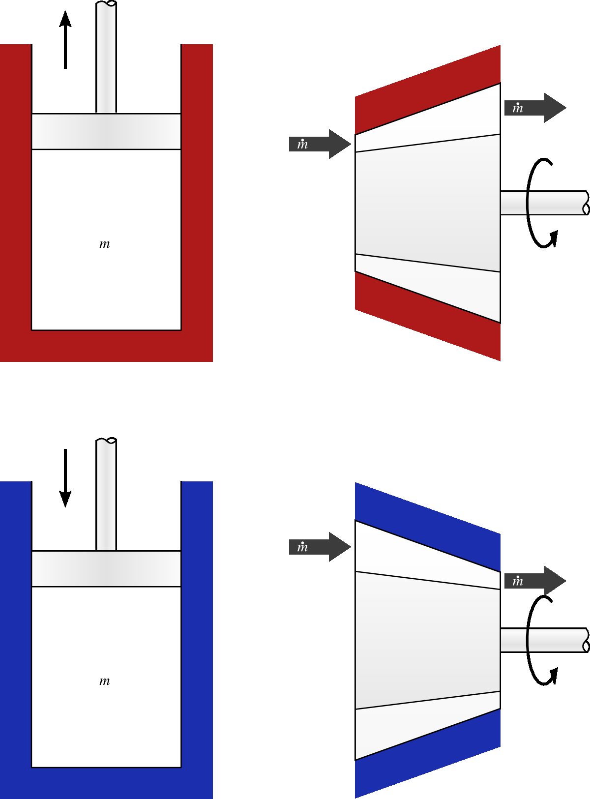
It is possible to heat or cool a gas while maintaining its temperature constant (figure 4.10). A process at constant temperature is called isothermal.

For an ideal gas, a process at constant temperature always occurs at constant energy. For each joule of heat supplied to the gas, one joule of work must be extracted from it; conversely, every heat withdrawal must be compensated by an equal amount of work input.

In practice, this complexity makes it so that isothermal heat transfers are rarely used in industry. However, they have crucial theoretical importance, which we will explore in chapter 7 (the second law).

When the temperature of an ideal gas remains constant, its properties vary according to the relation

p v = constant

(4/25)

In a closed system, we have $q_{1\rightarrow 2}+w_{1\rightarrow 2}= \Delta u$ , and if the process is reversible, heat and work can be related to the properties of the gas, although not without some difficulty.

Figure 4.10:A constant-temperature (isothermal) process undergone by an ideal gas. In a closed system (left), the gas is allowed to do work on a piston while being heated, and conversely, work is done on the gas when it is cooled. In an open system (right), the same manipulations are carried out continuously.

Diagram CC-0 Olivier Cleynen

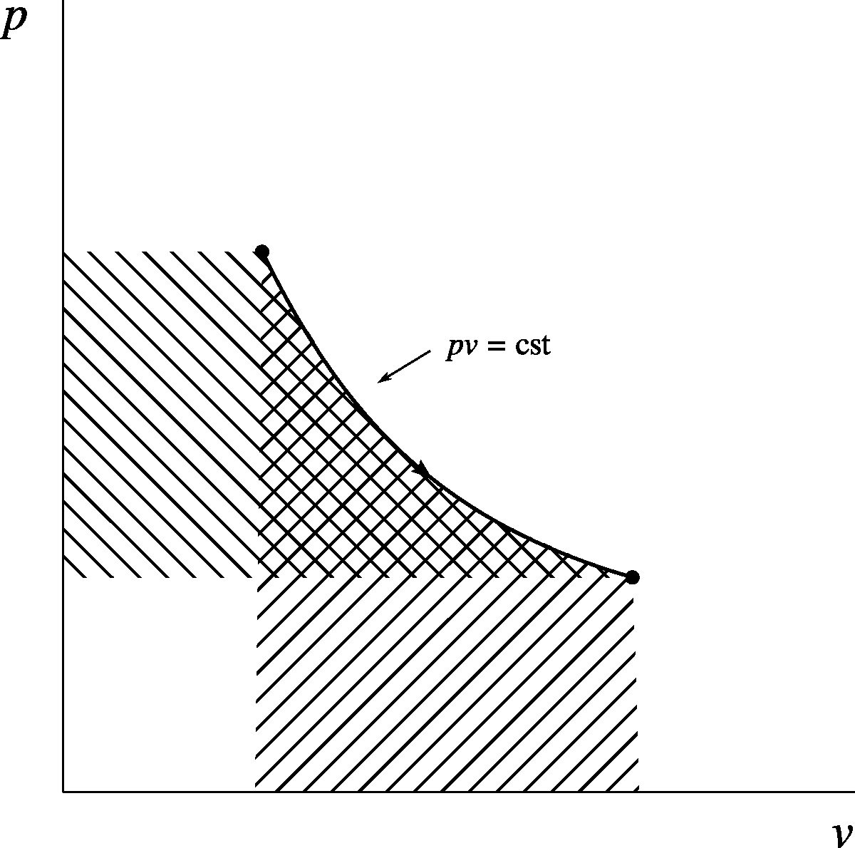
Figure 4.11:Expansion (heating) at constant temperature of an ideal gas, represented on a pressure-volume diagram.

Diagram CC-0 Olivier Cleynen

\begin{aligned} w_{1\rightarrow 2}&= -\int_{1}^{2} pdv = -\int_{1}^{2} \frac{R T_{\mathrm{cst}.}}{v}\, dv = -R T_{\mathrm{cst}.}\int_{1}^{2} \frac{dv}{v} \\ &= -R T_{\mathrm{cst}.}[\ln v]_{v_{1}}^{v_{2}} = R T_{\mathrm{cst}.}\ln \left(\frac{v_{1}}{v_{2}}\right) \end{aligned}

(15)

w_{1\rightarrow 2}= R T_{\mathrm{cst}.}\ln \left(\frac{v_{1}}{v_{2}}\right)

(4/26)

during a reversible process at constant temperature, in a closed system.

One can also express work in terms of pressure, since with equation 4/25, we have $\frac{v_{1}}{v_{2}} = \frac{p_{2}}{p_{1}}$ . Thus:

w_{1\rightarrow 2}= R T_{\mathrm{cst}.}\ln \left(\frac{p_{2}}{p_{1}}\right)

(4/27)

during a reversible process at constant temperature, in a closed system.

The heat transfer can be easily quantified. Indeed, the internal energy does not change:

q_{1\rightarrow 2}= \Delta u - w_{1\rightarrow 2}= 0 - w_{1\rightarrow 2}= -w_{1\rightarrow 2}

(4/28)

during a reversible process at constant temperature, in a closed system.

When the process occurs in an open system, we have $q_{1\rightarrow 2}+ w_{1\rightarrow 2}= \Delta h$ and, if the process is reversible, heat and work can be quantified in the same way:

\begin{aligned} w_{1\rightarrow 2}&= \int_{1}^{2} vdp = \int_{1}^{2} \frac{R T_{\mathrm{cst}.}}{p}\, dp = R T_{\mathrm{cst}.}\int_{1}^{2} \frac{dp}{p} \\ &= R T_{\mathrm{cst}.}[\ln p]_{p_{1}}^{p_{2}} = R T_{\mathrm{cst}.}\ln \left(\frac{p_{2}}{p_{1}}\right) = R T_{\mathrm{cst}.}\ln \left(\frac{v_{1}}{v_{2}}\right) \end{aligned}

(16)

w_{1\rightarrow 2}= R T_{\mathrm{cst}.}\ln \left(\frac{p_{2}}{p_{1}}\right) = R T_{\mathrm{cst}.}\ln \left(\frac{v_{1}}{v_{2}}\right)

(4/29)

during a reversible process at constant temperature, in an open system.

This relation, identical to equation 4/27, should not surprise the insightful student, since the $pv =$ constant relationship ensures that for two given points in figure 4.11, the area under the curve is always equal to the area to the left of the curve.

The heat transfer can be quantified without difficulty, of course:

q_{1\rightarrow 2}= \Delta h - w_{1\rightarrow 2}= 0 - w_{1\rightarrow 2}

(17)

q_{1\rightarrow 2}= -w_{1\rightarrow 2}

(4/30)

during a reversible process at constant temperature, in an open system.

Example 4.7

For air, we measure $c_{p (\mathrm{air})}= 1005 J kg^{-1}K^{-1}, c_{v (\mathrm{air})}= 718 J kg^{-1}K^{-1}$ , $R_{\mathrm{air}}= 287 J kg^{-1}K^{-1}$ . A mass of $2.5 kg (5.512 lb)$ of air in a reservoir is at a pressure of $2 bar (29.01 psi)$ and a temperature of $800^{\circ}C (1472 ^{\circ} F)$ . We want to supply it with $100 kJ$ of heat without changing its temperature. What should be the transfer of work? What will be the volume and pressure in the end?

The work is easy to determine: $W_{\mathrm{A}\rightarrow \mathrm{B}}+ Q_{\mathrm{A}\rightarrow \mathrm{B}}= \Delta U = 0$ here since the temperature does not change. Thus, $W_{\mathrm{A}\rightarrow \mathrm{B}}= -Q_{\mathrm{A}\rightarrow \mathrm{B}}= -100 kJ$ (the gas must provide as much work as it receives as heat). The final properties are obtained using equation 4/26:

w_{\mathrm{A}\rightarrow \mathrm{B}}= R T_{\mathrm{cst}.}\ln (\frac{v_{\mathrm{A}}}{v_{\mathrm{B}}}) = R T_{\mathrm{cst}.}\ln (\frac{V_{\mathrm{A}}}{V_{\mathrm{B}}})

(18)

\frac{V_{\mathrm{A}}}{V_{\mathrm{B}}} = \exp [\frac{w_{\mathrm{A}\rightarrow \mathrm{B}}}{R T_{\mathrm{cst}.}}] = \exp [\frac{W_{\mathrm{A}\rightarrow \mathrm{B}}}{m R T_{\mathrm{cst}.}}]

(19)

= \exp [\frac{-100 \times 10^{3}}{2.5 \times 287 \times (800 + 273.15)}] = 0.878207

(20)

And since $V_{\mathrm{A}}= \frac{m R T_{\mathrm{A}}}{p_{\mathrm{A}}}$ , we obtain a final volume $V_{\mathrm{B}}= \frac{V_{\mathrm{A}}}{0.878207}= 4.384 m^{3}= 1158 US gal$ . Finally, the final pressure is obtained by comparing the final and initial states: $p_{\mathrm{A}}V_{\mathrm{A}}= m R T_{\mathrm{A}}= m R T_{\mathrm{B}}= p_{\mathrm{B}}V_{\mathrm{B}}$ (or with equation 4/27): $p_{\mathrm{B}}= p_{\mathrm{A}} \frac{V_{\mathrm{A}}}{V_{\mathrm{B}}} = 2\times 10^{5}\times 0.878 207 = 1.756\times 10^{5}Pa = 1.756 bar = 25.47 psi$ .

The volume increases and the pressure decreases, since the gas is doing work while it receives heat.

It is difficult to hide that this type of process is rarely used in practice, but it will serve us to develop an extraordinary absolute thermometer-engine-refrigerator, in chapter 7 (the second law).

4.4.5 Reversible adiabatic processes¶

An adiabatic process is one where there is no heat transfer (figure 4.12). This can be achieved by wrapping the gas container or duct with a thick layer of thermal insulation.

Figure 4.12:A reversible adiabatic (isentropic) process undergone by an ideal gas. In a closed system (left) as well as in an open system (right), the apparatus is perfectly insulated, so that there is no heat transfer, even if the gas temperature varies.

A reversible adiabatic process is carried out infinitely slowly. A piston in a cylinder will need to be moved infinitely slowly for this, and a steady-flow compressor will need to be infinitely long. Later, in chapter 8 (entropy), we will call these processes isentropic.

It must be noted that even though there is absolutely no heat transfer, the temperature must necessarily vary in such a process, since the work is non-zero. This temperature change is often the intended effect, as we will see in chapter 7 (the second law).

In a closed system, we have $q_{1\rightarrow 2}+w_{1\rightarrow 2}= \Delta u$ and, if the process is reversible, heat and work are quantified without any difficulty:

q_{1\rightarrow 2}= 0

(4/31)

during a reversible adiabatic process, by definition.

w_{1\rightarrow 2}= \Delta u - q_{1\rightarrow 2}= \Delta u = c_{v}\Delta T

(4/32)

during a reversible adiabatic process in a closed system.

When the process occurs in an open system, we have $q_{1\rightarrow 2}+ w_{1\rightarrow 2}= \Delta h$ and we can also write:

q_{1\rightarrow 2}= 0

(4/33)

w_{1\rightarrow 2}= c_{p}\Delta T

(4/34)

during a reversible adiabatic process, in an open system.

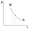
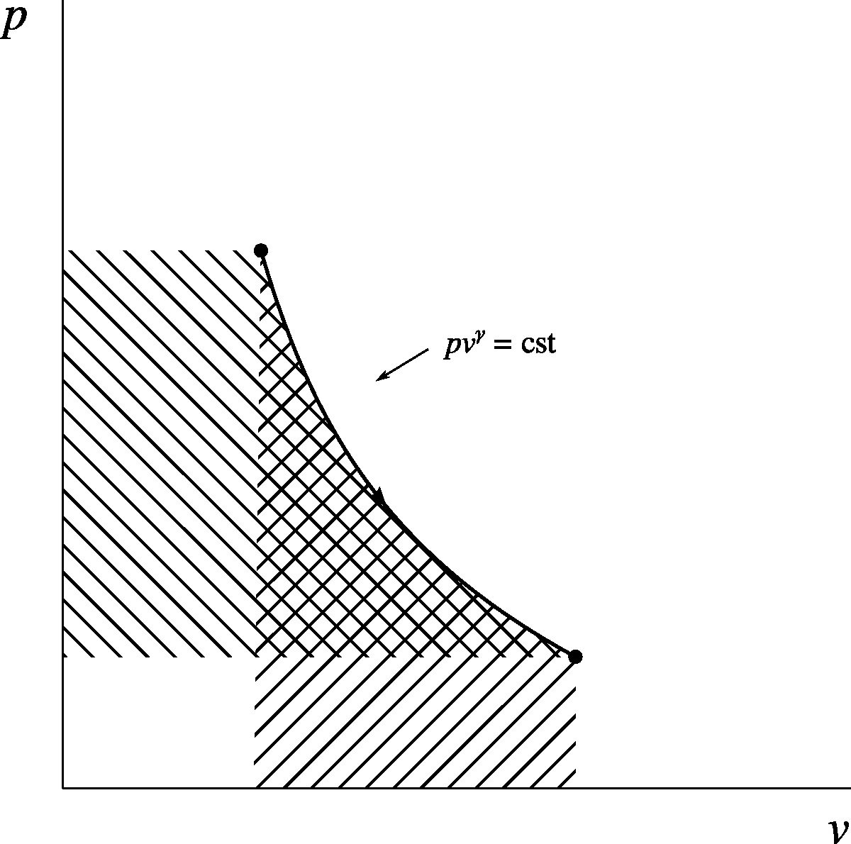
Figure 4.13:Reversible adiabatic expansion of an ideal gas, represented on a pressure-volume diagram.

Diagram CC-0 Olivier Cleynen

Unfortunately, these two equations 4/32 and 4/34 are of no use until we have predicted the temperature $T_{2}$ at the end of the process. However, in a reversible adiabatic process, nothing remains constant: the specific volume, pressure, and temperature all vary. How can we quantify these properties?

Let us start with an infinitely small adiabatic process in a closed system.

When the process is reversible, $δw = -pdv$ and then:

δ q = du - δ w = 0

(21)

du + pdv = 0

(22)

By using $du = c_{v}dT$ for an ideal gas and $p = RT/v$ , we can rewrite this equation as:

c_{v}dT + \frac{RT}{v} dv = 0

(23)

\frac{1}{T} dT + \frac{R}{c_{v}} \frac{1}{v} dv = 0

(24)

By integrating between two states 1 and 2:

\ln (\frac{T_{2}}{T_{1}}) + \frac{R}{c_{v}} \ln (\frac{v_{2}}{v_{1}}) = 0

(25)

\ln (\frac{T_{2}}{T_{1}}) + \ln \left(\frac{v_{2}}{v_{1}}\right) ^{\frac{R}{c_{v}}} = 0

(26)

\ln (\frac{T_{2}}{T_{1}}) = \ln \left(\frac{v_{1}}{v_{2}}\right) ^{\frac{R}{c_{v}}}

(4/35)

And since $R = c_{p}- c_{v}$ (equation 4/8) and $\gamma \equiv c_{p}/c_{v}$ (equation 4/9), we have $\frac{R}{c_{v}} = \gamma - 1$ , which allows us to reformulate equation 4/35 above as:

\left(\frac{T_{2}}{T_{1}}\right) = \left(\frac{v_{1}}{v_{2}}\right) ^{\gamma -1}

(27)

Thus, we have linked temperature and specific volume when the process is reversible adiabatic (devoid of heat transfer and infinitely slow).

Some algebraic manipulations, which are left to the student to revise, allow us to derive this expression in terms of pressure. We thus obtain the following three relations:

\left(\frac{T_{1}}{T_{2}}\right) = \left(\frac{v_{2}}{v_{1}}\right) ^{\gamma -1}

(4/36)

\left(\frac{T_{1}}{T_{2}}\right) = \left(\frac{p_{1}}{p_{2}}\right) ^{\frac{\gamma -1}{\gamma}}

(4/37)

\left(\frac{p_{1}}{p_{2}}\right) = \left(\frac{v_{2}}{v_{1}}\right) ^{\gamma}

(4/38)

for any reversible adiabatic process.

This last equation 4/38 is equivalent to the expression:

p v^{\gamma}= constant

(4/39)

for any reversible adiabatic process.

Example 4.8

For air, we have $c_{p (\mathrm{air})}= 1005 J kg^{-1}K^{-1}, c_{v (\mathrm{air})}= 718 J kg^{-1}K^{-1}, R_{\mathrm{air}}= 287 J kg^{-1}K^{-1}$ , and $\gamma _{\mathrm{air}}= 1.4$ . A compressed air tank of $200 L (52.83 US gal)$ contains air at 40 bar and $50^{\circ}C (580.2 psi$ and $122 ^{\circ} F)$ . The ambient atmosphere is at $1 bar (14.5 psi)$ . What is the maximum amount of work that can be extracted from the compressed air without supplying heat?

The maximum work will be obtained if the expansion is reversible. Since we are not allowed to supply heat, our best option here is to perform a reversible adiabatic expansion from 40 bar to 1 bar. We want to calculate the final temperature, since it will give us the change in energy, thus the work done by the gas. Among the three daunting relations 4/36 to 4/38, it is the second one that interests us:

With $\left(\frac{T_{\mathrm{A}}}{T_{\mathrm{B}}}\right) = \left(\frac{p_{\mathrm{A}}}{p_{\mathrm{B}}}\right)^{\frac{\gamma-1}{\gamma}}$ . Thus: $T_{\mathrm{B}}= T_{\mathrm{A}}\left(\frac{p_{\mathrm{A}}}{p_{\mathrm{B}}}\right) ^{-\frac{\gamma-1}{\gamma}}= (50 + 273.15) ( \frac{40}{1} )^{-\frac{1.4-1}{1.4}} = 112.6 K = -160.5^{\circ}C = -257 ^{\circ} F$ . The work done by the closed system composed of the gas is therefore $w_{\mathrm{A}\rightarrow \mathrm{B}}= \Delta u - q_{\mathrm{A}\rightarrow \mathrm{B}}= c_{v}\Delta T - 0 = 718 \times (-160.5 - 50) = -1.5115 \times 10^{5}J kg^{-1}= -151.1 kJ kg^{-1}$ . By calculating the mass $m_{\mathrm{A}}= \frac{p_{\mathrm{A}}V_{\mathrm{A}}}{R T_{\mathrm{A}}} = \frac{40\times 10^{5}\times 0.2}{287\times (50+273.15)}= 8.626\,\mathrm{kg}$ , we obtain $W_{\mathrm{A}\rightarrow \mathrm{B}}= m_{\mathrm{A}}w_{\mathrm{A}\rightarrow \mathrm{B}}= 8.626 \times -151.1 \times 10^{3}= -1.3038 \times 10^{6}J = -1.304 MJ$ .

This amount of energy is enough to accelerate, without friction, a vehicle weighing $1 t$ to a speed $C = \left[\frac{1.3038\times 10^{6}}{\frac{1}{2}\times 1000}\right]^{0.5} = 51.1 m s^{-1}\approx 180 km/h \approx 114 mph$ .

The final temperature, $-160^{\circ}C$ (!), reminds us not to confuse

“adiabatic” with “constant temperature”.

In the fractions, the pressures can be left in bars or $psi$ , but the temperatures cannot remain in $^{\circ}C$ or $^{\circ} F$ .

The expansion corresponds to the maximum work because it is reversible. If it were not reversible, then the temperature of the gas would drop less and the work would be lower (we would still have $w = c_{v}\Delta T)$ . In the most extreme case, that of Joule and Gay-Lussac’s expansion (§4.3.2), the temperature would remain at $50^{\circ}C$ and no work would be done.

4.4.6 Arbitrary processes¶

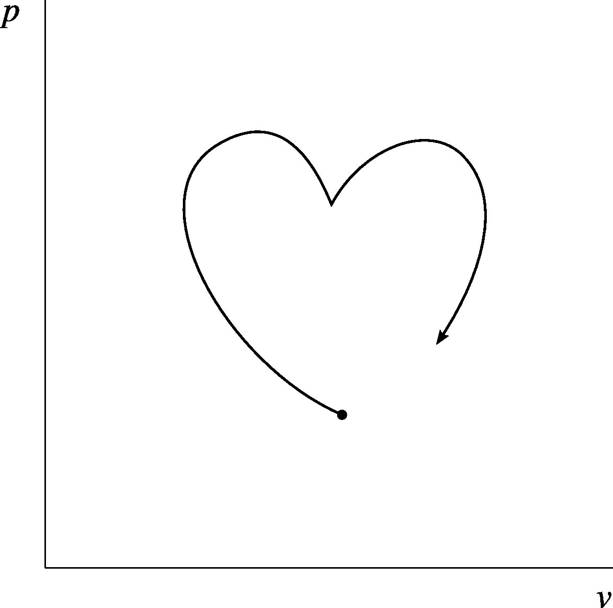
It is important to keep in mind that in practice, the properties of a gas can be changed in any arbitrary manner (figure 4.14).

Figure 4.14:An entirely arbitrary process undergone by an ideal gas represented on a pressure-volume diagram. Such a process requires a complex combination of heat and work transfers, which the student is invited to conceptualize.

CC-0 Olivier Cleynen

We have focused on four specific processes of ideal gases, since each plays an important role for physicists and engineers in the design of thermal machines. However, this should not limit our way of thinking about a gas or the changes it may undergo. By cleverly controlling heat and work transfers, we can certainly cause any arbitrary process.

A Bit of History

Lavoisier and Laplace’s Inquiries

By Philippe Depondt

Pierre and Marie Curie University, Paris

The debates on the nature of heat continued until the end of the 19th century with the gradual acceptance of atomic theories. An important step in this reflection is succinctly and eloquently presented in the Mémoire sur la chaleur (Memoir on Heat), 1780 [1] by the French physicists Lavoisier and Laplace:

“Physicists are divided on the nature of heat.

Many among them regard it as a fluid spread throughout nature, and of which bodies are more or less penetrated, according to their temperature and their particular disposition to retain it; it can combine with them, and, in this state, it ceases to act on the thermometer and to transfer from one body to another; it is only in the state of freedom, which allows it to establish equilibrium within bodies, that it forms what we call free heat.

Other physicists think that heat is merely the result of the imperceptible movements of the molecules of matter. It is known that bodies, even the densest ones, are filled with a great number of pores or small voids, whose volume can considerably surpass that of the matter they contain; these empty spaces allow their imperceptible parts the freedom to oscillate in all directions, and it is natural to think that these parts are in continual agitation, which, if it increases to a certain point, can disunite and decompose bodies; it is this internal motion which, according to the physicists we speak of, constitutes heat.

To develop this hypothesis, we shall observe that, in all movements where there is no abrupt change, there exists a general law which geometers have designated under the name of the principle of the conservation of vis viva; this law consists in that, in a system of bodies acting upon each other in any manner, the vis viva, that is to say, the sum of the products of each mass by the square of its velocity, remains constant. If the bodies are driven by accelerating forces, the vis viva is equal to what it was at the origin of the movement, plus the sum of the masses multiplied by the squares of the velocities due to the action of the accelerating forces. In the hypothesis we are examining, heat is the vis viva resulting from the imperceptible movements of the molecules of a body; it is the sum of the products of the mass of each molecule by the square of its velocity.

If one brings into contact two bodies whose temperatures are different, the quantities of motion they will mutually communicate will initially be unequal; the vis viva of the colder body will increase by the same amount by which the vis viva of the other will decrease, and this increase will continue until the quantities of motion communicated from one to the other are equal; in this state, the temperature of the bodies will have reached uniformity.

This way of regarding heat easily explains why the direct impulse of solar rays is negligible, while they produce a great amount of heat. Their impulse is the product of their mass by their simple velocity; now, although this velocity is excessive, their mass is so small that this product is almost nil, whereas their vis viva, being the product of their mass by the square of their velocity, represents heat of an order much superior to that of their direct impulse. This impulse on a white body, which abundantly reflects light, is greater than on a black body, and yet the solar rays communicate less heat to the former because these rays, by being reflected, carry away their vis viva, which they communicate to the black body that absorbs them.

We will not decide between the two preceding hypotheses; several phenomena seem to favor the latter; such is, for example, that of the heat produced by the friction of two solid bodies; but there are others that are more simply explained by the former; perhaps both occur simultaneously. In any case, since one can only form these two hypotheses regarding the nature of heat, one must accept the principles common to both; thus, according to both, the quantity of free heat always remains the same in the simple mixing of bodies.

This is evident if heat is a fluid that tends to reach equilibrium, and if it is merely the vis viva resulting from the internal motion of matter, the principle in question follows from the principle of the conservation of vis viva. The conservation of free heat in the simple mixing of bodies is thus independent of any hypothesis regarding the nature of heat; it has been generally accepted by physicists, and we shall adopt it in the following research.”

At the time when this text was written, the atomic hypothesis remained largely speculative due to the lack of adequate experimental means: the experiment by Jean Perrin that finally settled the issue only took place in the early years of the 20th century, and the X-ray diffraction experiments suggested by Max von Laue occurred in 1912.

Problems¶

Air is considered an ideal gas.

$c_{v (\mathrm{air})}= 718 J kg^{-1}K^{-1} \qquad R_{\mathrm{air}}= 287 J kg^{-1}K^{-1}$

$c_{p (\mathrm{air})}= 1005 J kg^{-1}K^{-1} \qquad \gamma _{\mathrm{air}}= 1.4$

We assume that for a reversible adiabatic process (without heat transfer and infinitely slow), the properties of air are linked according to the following three relationships:

\left(\frac{T_{1}}{T_{2}}\right) = \left(\frac{v_{2}}{v_{1}}\right)^{\gamma -1}

(4/36)

\left(\frac{T_{1}}{T_{2}}\right) = \left(\frac{p_{1}}{p_{2}}\right)^{\frac{\gamma -1}{\gamma}}

(4/37)

\left(\frac{p_{1}}{p_{2}}\right) = \left(\frac{v_{2}}{v_{1}}\right)^{\gamma}

(4/38)

We also assume that during a reversible isothermal process (at constant temperature and infinitely slow) of an ideal gas, the work done in an open or closed system is:

w_{1\rightarrow 2}= RT_{\mathrm{cst}.}\ln \left(\frac{p_{2}}{p_{1}}\right) = RT_{\mathrm{cst}.}\ln \left(\frac{v_{1}}{v_{2}}\right)

(4/29)

Exercise 4.2

Heating of an Air Tank A compressed air tank made out of sealed concrete has a fixed volume of $1.2 m^{3}$ . Air is stored in it at a pressure of 2 bar. The tank is placed in the sun and solar heating raises the temperature from $5^{\circ}C$ to $60^{\circ}C (41 ^{\circ} F$ to $140 ^{\circ} F)$ . 1. What are the mass, specific volume, density, and pressure inside the tank, before and after heating? When the temperature reaches $60^{\circ}C$ , a valve opens and lets air escape to bring the pressure in the tank back down to the initial pressure of $2 bar (29 psi$ . During the release, the temperature of the air inside the tank remains constant. 2. How much air mass should be allowed to escape? When the pressure has reached 2 bar, the valve closes and the tank, once again sealed, cools slowly at constant volume. The final temperature returns to $5^{\circ}C$ . 3. What is the final pressure in the tank?

Answer

$m_{1}= \frac{p_{1}V_{1}}{RT_{1}} = 3.006 kg$ ; $v_{1}= 0.3991 m^{3}kg^{-1}$ ; $\rho _{1}= 2.505 kg m^{-3}$ ; $p_{1}= 2 bar$ ; $m_{2}= m_{1}; v_{1}= v_{2}; \rho _{1}= \rho _{2}; p_{2}= \frac{RT_{2}}{v_{2}} = 2.395bar.$
$m_{3}= 2.51 kg$ , thus $m_{\mathrm{exhaust}}= m_{3}-m_{2}0.4959 kg$ ; $3) p_{4}= \frac{RT_{4}m_{4}}{V_{4}} = 1.67bar.$

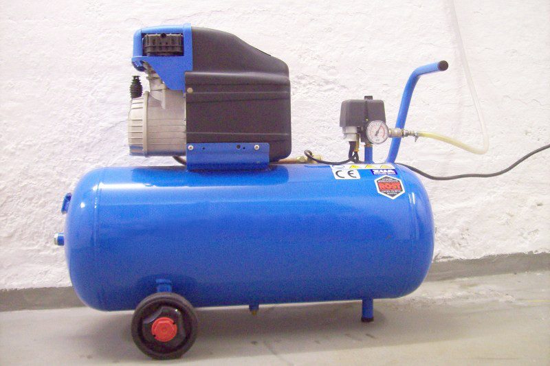
Figure 4.15:A small electric compressor mounted on a portable air tank

Exercise 4.5

Turbine of a Turbojet Engine A student disassembles the Turboméca Marboré turbojet engine from a Fouga Magister in order to study and modify its operation. S/he operates the engine on a test bench. At the inlet of the turbine, the conditions are measured at $110 m s^{-1}(246 mph)$ and $1000^{\circ}C (1832 ^{\circ} F)$ . At the outlet of the turbine, these properties are measured at $125 m s^{-1}(279.6 mph)$ and $650^{\circ}C (1202 ^{\circ} F)$ . The student also measures the heat losses from the turbine as $75 kJ kg^{-1}$ . 1. What is the specific power delivered by the turbine? 2. What condition must the student maintain to obtain a power of $1 MW$ ?

Answer

With equation 3/15, $w_{\mathrm{turbine}}= c_{p}(T_{\mathrm{B}}- T_{\mathrm{A}}) + \frac{1}{2}(C_{\mathrm{B}}^{2}- C_{\mathrm{A}}^{2}) - q_{\mathrm{A}\rightarrow \mathrm{B}}= -275 kJ kg^{-1}$
$\dot{m}= \frac{\dot{W}_{\mathrm{turbine}}}{w_{\mathrm{turbine}}} = 3.64 kg s^{-1}$

Exercise 4.6

Elementary Processes: Isothermal Compression A mass of $3.5 kg (7.716 lb)$ of air is compressed reversibly in an isothermal manner (constant temperature) from $2 bar$ and $15^{\circ}C$ to $45 bar$ (from $29.01 psi$ and $59^{\circ} F$ to $652.7 psi)$ 1. Draw the process qualitatively (that is, without showing numerical values) on a pressure-volume diagram. 2. What are the amounts of work and heat involved? 3. If the compression were carried out in a reversible adiabatic manner, would the final volume be different?

Answer

With equation 4/26, $w_{1\rightarrow 2}= +257.58 kJ kg^{-1}$ (so, an amount of work received); $W_{1\rightarrow 2}= +901.2 kJ$ ; $Q_{1\rightarrow 2}= -W_{1\rightarrow 2}$ (so, an amount of heat expended)
Yes, we would have $v_{2 \mathrm{ad.rev}.}= v_{1}\left(\frac{p_{1}}{p_{2}}\right)^{\frac{1}{\gamma}} > v_{2 \mathrm{isoth}.}= v_{1}\left(\frac{p_{1}}{p_{2}}\right)$ .

Exercise 4.7

Elementary Processes: Isobaric and Isochoric Coolings A mass of $2 kg$ of air in a deformable reservoir is at a pressure of $4.5 bar (65.27 psi)$ and occupies a volume of $800 L (211.3 US gal)$ . It is cooled, and the reservoir maintains constant pressure until the volume has been reduced by $40\%$ . After this, the cooling is continued at constant volume until the temperature reaches $25^{\circ}C (77 ^{\circ} F)$ . 1. Sketch the process on a pressure-volume diagram. 2. What is the work done by the air? 3. What is the heat cost for the entire process?

Answer

$W_{1\rightarrow 3}= -\int_{1}^{2} pdV - \int_{2}^{3} pdV = -p_{\mathrm{cst}.}\Delta V - 0 = +144 kJ$
$Q_{1\rightarrow 3}= U_{3}- U_{1}- W_{1\rightarrow 3}= mc_{v}\left(T_{3}- \frac{p_{1}V_{1}}{mR}\right) - W_{1\rightarrow 3}= -616.5 kJ$

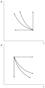
Figure 4.16:Elementary processes undergone by a perfect gas

Exercise 4.11

**Compressor of a Turbofan Inside one of the engines of a commercial aircraft, the compressor (figure 4.17) is almost adiabatic. During cruise at $33 000 ft$ , the atmosphere is at $-50^{\circ}C (-58 ^{\circ} F)$ and $0.25 bar (3.626 psi)$ . The fan is driven by the turbine through a mechanical shaft. It receives $55 kg s^{-1}$ of air at atmospheric conditions, and compresses this flow up until $8 bar (116 psi)$ . 1. Starting from the following relation,

\left(\frac{p_{1}}{p_{2}}\right) = \left(\frac{v_{2}}{v_{1}}\right)^{\gamma}

(4/38)

valid for a reversible adiabatic process undergone by a perfect gas, show (without using equation 4/36) that:

\left(\frac{T_{1}}{T_{2}}\right) = \left(\frac{p_{1}}{p_{2}}\right)^{\frac{\gamma -1}{\gamma}}

(4/37)

What is the minimum theoretical power to be supplied to the compressor? 3. Under what conditions would this power be obtained? In reality, the compressor requires significantly more power to operate. We model the actual process inside the compressor with two distinct phases: • A heating at constant pressure, conducted by friction, with power representing $15 \%$ of the theoretical power calculated earlier; • Then, an ideal compression up to 8 bar. 4. Compare the theoretical compression from question 2 and this new process on a pressure-volume diagram. Graphically represent the work done on one of the processes. 5. What is the power supplied to the compressor in this new scenario? under license by Sulzer in Switzerland Photo CC-by-sa Sulzer AG**

Answer

Replace $v_{2}$ with $\frac{RT_{2}}{p_{2}}$ , do the same with $v_{1}$ . Work out the algebra and the result will come naturally;
With eq. 4/37, we obtain $T_{\mathrm{B}}= 600.7 K$ , thus $W_{\mathrm{A}\rightarrow \mathrm{B}}= +20.87 MW$ ;
see §4.4.5 p. 100;
$T_{\mathrm{C}}= 279.8 K$ ; $T_{\mathrm{D}}= 753.1 K$ ; thus $W_{\mathrm{real} \mathrm{compressor}}=\dot{W}_{\mathrm{friction} \mathrm{losses} \mathrm{A}\rightarrow \mathrm{C}}+\dot{W}_{\mathrm{C}\rightarrow \mathrm{D}}= +29.29 MW (+40 \%)$ .

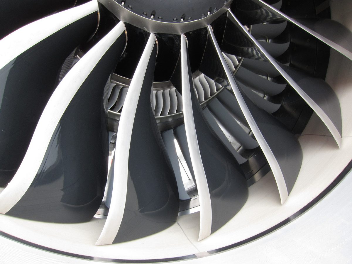
Figure 4.17:Air intake of one of the four General Electric GEnx-2B turbofans equipping a Boeing 747-8. The two-color fan blades are visible in the foreground; behind, the air flow is divided between the compressor inlet (internal) and the cold flow rectifier stators (external).

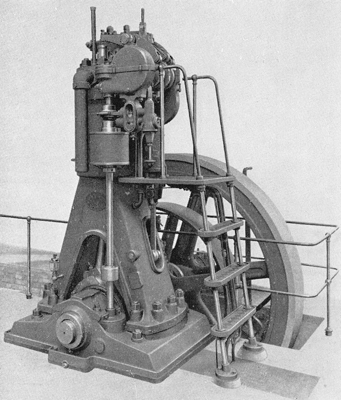
Figure 4.18:Diesel Engine from 1898, manufactured under license by Sulzer in Switzerland

Exercise 4.12

Compression and Combustion in a Diesel Engine In 1890, a young German engineer with a passion for thermodynamics (§7.6) developed a low-power, low-speed, and high-efficiency engine in a laboratory (figure 4.18). The engine was designed to be robust and simple; it had only one cylinder. Here, we study part of its operating cycle. The piston inside the cylinder periodically varies the volume between $3 L$ (bottom dead center, piston at the bottom of its stroke) and $0.3 L$ (top dead center, piston at the top of its stroke). The engine starts its cycle at bottom dead center, when it is filled with air at $20^{\circ}C$ and $1 bar (68 ^{\circ} F$ and $14.5 psi)$ . The piston compresses this air to top dead center. The compression is done reversibly (very slowly), but non-adiabatically: the air receives heat through the walls throughout the process. The engineer predicted that its properties would vary according to the relation $p v^{1.5}=$ constant. 1. The work done by a force $\vec{F}$ along a displacement $l$ is expressed as $W \equiv \vec{F} \cdot \vec{l}$ (equation 1/10). Starting from this equation, express the work done on a fixed mass body in terms of its specific volume and internal pressure. 2. How much energy in the form of work will the gas compression have cost? 3. How much energy in the form of heat will the gas have received during compression? When the piston reaches the top of its stroke, fuel is progressively injected into the cylinder to allow for combustion to occur. The amount of injected fuel provides for a total heat input of $2 kJ$ . The combustion takes place at constant pressure. 4. Draw the processes undergone by the gas during compression and combustion on a pressure-volume diagram, qualitatively (that is, without showing numerical values). 5. What will be the maximum temperature reached within the engine? 6. In order to avoid structural failure, the engineer must ensure that the force transmitted by the piston never exceeds $10 kN (2248 lbf)$ . What constraint must be respected for this?

Answer

see §1.3 p. 16 & §2.4.1 p. 36;
$W_{\mathrm{A}\rightarrow \mathrm{B}}= -m\int ^{\mathrm{B}}_{\mathrm{A}}pdv = +1.298 kJ$
$p_{\mathrm{B}}= kv_{\mathrm{B}}^{-1.5}= 31.6 bar$ , we have $T_{\mathrm{B}}= 926.3 K$ . Then, $Q_{\mathrm{A}\rightarrow \mathrm{B}}= \Delta U -W_{\mathrm{A}\rightarrow \mathrm{B}}= +0.3254 kJ$ .
With constant pressure, with equation 4/17, $T_{\mathrm{C}}= \frac{Q_{\mathrm{B}\rightarrow \mathrm{C}}}{m c_{p}} + T_{\mathrm{B}}= 1483.7 K (1211^{\circ}C)$ .
$A_{\max}= \frac{F_{\max}}{p_{\mathrm{B}}} = 3.164 \times 10^{-3}m^{2}$ (diameter $D_{\max}= 6.35 cm)$ .

Exercise 4.13

Turbojet Engine

An early 1960s military aircraft is equipped with a turbojet engine (figure 4.19). We wish to calculate the theoretical maximum speed at which it could accelerate the air at the nozzle outlet. The engine is tested on a stationary test bench. When air passes through the turbojet engine, it goes through four components that we will model as if they were ideal:

The compressor (figure 4.20) compresses the air adiabatically and reversibly. At the inlet, the air is at 0.9 bar and $5^{\circ}C$ ; at the outlet, the pressure is increased to 19 bar.

The combustion chamber allows for the heating of air while maintaining its pressure constant. At the outlet of the combustion chamber, the temperature has been increased to $1100^{\circ}C$ .

The turbine extracts energy from the air to power the compressor. In the turbine, the air expands adiabatically and reversibly.

The nozzle is a component in which no power is added or extracted from the air. As it flows across the nozzle, the air expands adiabatically and reversibly; its speed increases significantly. At the outlet of the nozzle, it has returned to atmospheric pressure and is expelled into the atmosphere.

The goal of the problem is to calculate the speed at which the turbojet engine is capable of releasing the air.

Starting from the following relation,

\left(\frac{T_{1}}{T_{2}}\right) = \left(\frac{v_{2}}{v_{1}}\right)^{\gamma -1}

(4/36)

valid for a reversible adiabatic process undergone by a perfect gas, show (without using equation 4/38) that:

\left(\frac{T_{1}}{T_{2}}\right) = \left(\frac{p_{1}}{p_{2}}\right)^{\frac{\gamma -1}{\gamma}}

(4/37)

What is the air temperature at the compressor outlet?
What is the specific power supplied to the compressor?
What is the specific power supplied in the form of heat in the combustion chamber?
What must be the temperature at the turbine outlet for it to power the compressor?
What will then be the pressure at the turbine outlet?
What will be the exhaust gas temperature at the nozzle outlet?
Finally, what will be the gas ejection speed at the nozzle outlet?
Draw the complete series of processes on a pressure-volume diagram, qualitatively.
On the same pressure-volume diagram, plot the processes that the gas would follow if the compressor could not compress the air reversibly (real compressor, compression with internal friction).

Answer

With equation 4/37, $T_{\mathrm{B}}= 664.83 K$ ; 3) With equation 3/15, $w_{\mathrm{compressor}}= w_{\mathrm{A}\rightarrow \mathrm{B}}= +388.61 kJ kg^{-1}$ ; 4) $T_{\mathrm{C}}= 1373.15 K$ ; thus $q_{\mathrm{combustion}}= q_{\mathrm{B}\rightarrow \mathrm{C}}= +711.86 kJ kg^{-1}$ ; 5) Since $w_{\mathrm{turbine}}= -w_{\mathrm{compressor}}$ , we have $T_{D}= 986.47 K$ ; 6) With equation 4/37, $p_{\mathrm{D}}= 5.97 bar$ ; 7) Idem, with equation 4/37, $T_{\mathrm{E}}= 574.49 K$ ; 8) With equation 3/15, $C_{\mathrm{E}}= (-2\Delta h)^{\frac{1}{2}} = 909.98 m s^{-1}$ . Of course, these values do not account for the irreversibilities in an actual turbojet. These effects are approached in problem 4.11 p. 108 and formalized in chapter 10 (air-based power cycles).

Figure 4.19:Schematic of a turbojet engine. Air flows through the machine from left to right.

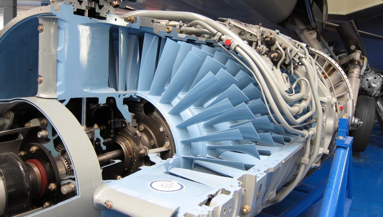
Figure 4.20:Compressor of a dissected snecma Atar turbojet engine (1948). Air flows from the left to the center of the image.

Diagram CC-by-sa Olivier Cleynen

Footnotes¶

Sometimes in other books, the constant in $J K^{-1}kg^{-1}$ is denoted as $r$ . The quantity then denoted $R = 8.3143 J K^{-1}mol^{-1}$ is universal, and gases adopt different values of $r$ depending on their molar mass $M \equiv \frac{m}{n}$ . In this book, we do not quantify amounts of substance.
↩