8. Entropy - Engineering Thermodynamics

8. Entropy¶

Entropy

The Terrifying Prophecy of Professor Clausius

Introduction¶

We present here the most powerful and difficult concept of thermodynamics.

This chapter 8 (entropy) aims to approach it in the most pragmatic way possible, starting from two questions:

• What does entropy represent?

• Why do physicists and engineers quantify its variations?

8.1 The Concept of Entropy¶

8.1.1 What is entropy used for?¶

At the very beginning of chapter 1 (fundamental concepts), we had seen that we could conceptualize energy as “a quantity that never changes when things evolve”. Thus, we quantify energy to determine the limits of what is possible: for example, we know that with $500 J$ , a stationary body of mass $10 kg$ cannot reach a speed greater than $10 m s^{-1}$ (eq. 1/5 p. 15).

However, our intuition and daily experience teach us that many transformations can only occur in one direction (figure 8.1). For example, there is as much energy in a glass of water on the edge of a table as in the same glass shattered with the water spilled on the floor. Yet we know, or more precisely, we have a deep conviction, that it is possible for the glass to fall and break, but impossible for the shards and water on the floor to spontaneously gather together into a full glass on the table. Thus, the quantification of energy is not entirely sufficient to determine what is possible. We would also like to be able to predict absolutely and quantitatively the direction in which energy can or cannot be transformed.

Entropy was conceived to address this question. By the end of this chapter, we will have a tool to calculate the direction of a process, that is, to mathematically predict which of two situations separated in time must have occurred before the other.

Figure 8.1:We have the intuition and an inner conviction that these three photos were taken in a very particular order. A calculation of the *entropy* in these three situations, in which the *energy* is the same, allows us to determine this order by associating a calculable quantity with our intuition.

images derived from Photos CC-by-sa by Jarosław W. Tuszyński

8.1.2 How can we determine the direction of a¶

process?¶

In the vocabulary of thermodynamics, the concept of a “one-way change” is of course called irreversibility. We had already discussed irreversibility in section §2.4.3, where we had determined that it had two main causes:

• The conversion of work into heat, through friction and turbulence;

• The transfer of a quantity of heat between two bodies at different temperatures.

Irreversible processes in fluids invariably lead to states where the temperature, pressure, or volume are greater than they would have been with a reversible process.

In order to quantify the irreversibility of a process, we will quantify the amount of heat that one would need to remove from the body to bring it back to its initial state reversibly. By subtracting to this amount the heat that was actually transferred, we obtain the heat that was somehow needlessly created during the process. Moreover, the lower the temperature at which this heat is created, and the less of it can be transformed into work (§7.5.1). We will thus “penalize” the heat cost by dividing it by the temperature. In this way, we will obtain a quantity in joules per kelvin – the entropy created during the process – which will be zero during reversible processes and will always be positive during irreversible processes. It is this creation that will be the unmistakable sign that the process is possible only in one direction.

8.2 Definition¶

8.2.1 Entropy is a property¶

Let us begin by acknowledging the fact that entropy is a physical property, meaning something that characterizes the state of a system. Put another way: if we consider a portion of the universe at a given moment (a system), we find that this system has a mass, a volume, a temperature: these quantities describe its current state (which is why they are called state quantities). Entropy is one of these quantities.

By contrast, we could say that heat, work, or electric current are not properties: they are not quantities that describe an object, but rather a transfer between two objects (path quantities).

Therefore, we will always think of entropy as the entropy “of something” (perhaps as we would say the color, the temperature “of something”). For example, we will say “this body has entropy” or “the entropy of this body is increasing/decreasing”, and not “we are taking/giving entropy to this body”. Rigorously, we say that entropy is an additive state quantity (see the appendices A3 and A4).

8.2.2 Definition¶

Entropy, noted $S$ , is a physical property.

• When a system undergoes a reversible process, its entropy varies such that:

dS \equiv \left(\frac{\mathrm{δ}Q}{T}\right)_{\mathrm{rev}.}

(8/1)

where the subscript rev. indicates the calculation is done along a reversible path; $dS$ is the infinitesimal change in entropy $(J K^{-1})$ ; δ $Q$ is the infinitesimal amount of (reversibly) supplied heat $(J)$ ;

and $T$ is the temperature at which the heat transfer occurs $(K)$ .

When it transitions from a state A to a state B reversibly, the entropy of a system therefore varies by an amount $\Delta S$ :

\Delta S = \int _{\mathrm{A}}^{\mathrm{B}} \left(\frac{\mathrm{δ}Q}{T}\right)_{\mathrm{rev}.}

(8/2)

where the subscript rev. indicates the calculation is done along a reversible path.

• When a system undergoes an irreversible process between A and B (as is the case for the majority of real processes), then a reversible path between these two states must be found and the integration 8/2 must be performed along it to calculate $\Delta S$ .

There is always a reversible way (in fact, there is even an infinity of such ways) to make a system undergo a process between two arbitrary states. For this, the work transfers must be carried out infinitely slowly and the heat transfers must be carried out with infinitesimal temperature differences.

We must be careful here: if one integrates the quantity $\frac{\delta Q}{T}$ along a process where the temperature or pressure are not homogeneous (for example during a rapid expansion, or in a body that has an internal temperature gradient, see §2.4.3), then a result will be obtained which is lower than the actual entropy change $\Delta S$ .

The SI unit of entropy $S$ is the $J\,K^{-1}$ (joule per kelvin); and correspondingly, the specific entropy $s$ is defined as:

s \equiv \frac{S}{m}

(8/3)

where $m$ is the considered mass $(kg)$ , and $s$ is its specific entropy $(J K^{-1}kg^{-1})$ .

In practice, the term “entropy” is often used even if it refers to specific entropy; the symbol and context determine which variable is being referred to.

Example 8.1

We extract $2000 J$ as heat, reversibly, from a mass of air while maintaining its temperature constant at $30^{\circ}C$ . How much does its entropy change?

Since the process is reversible, we immediately apply equation 8/2:

$\Delta S = S_{B}- S_{A}= \int _{\mathrm{A}}^{\mathrm{B}}\left(\frac{\delta Q}{T}\right)_{\mathrm{rev}.}= \left[\frac{1}{T_{\mathrm{cst}}}\int _{\mathrm{A}}^{\mathrm{B}}\delta Q\right]_{\mathrm{rev}.}= \left[\frac{1}{T_{\mathrm{cst}}}Q_{\mathrm{A}\rightarrow \mathrm{B}}\right]_{\mathrm{rev}.}=$

$\frac{1}{30+273.15}(-2000) = -6.6 J K^{-1}$ .

We have already explored reversible processes at constant temperature (isothermal processes) in sections §4.4.4 p. 98 and §5.4.4 p. 135. Here, the gas loses $2 kJ$ of heat and receives $2 kJ$ of work.

We do not know the value of entropy, but we know that it decreases by 7 joules per kelvin.

The change in entropy should not be confused with the thermal capacity, $c \equiv \frac{\mathrm{δ}q}{dT} = \frac{1}{m} \frac{\mathrm{δ}Q}{dT}$ (equation 1/16), where we divide the heat by the change in temperature. In this process, the thermal capacity is infinite since $dT = 0 K$ .

Once the cooling is done, the air is allowed to expand suddenly: the expansion is irreversible. During this process, only $1000 J$ is supplied as heat and only $1000 J$ is recovered as work. At the end of the expansion, the gas is in the same state (same temperature, pressure, and internal energy) as at the very beginning of the experiment. What is the entropy change?

This time, the process is not reversible. We should not consider the heat that is actually transferred, but the heat that would have been transferred in a reversible process leading to the same final state.

Fortunately, we know that the gas returns from B to its initial state A; and from A to B the process was reversible. By performing the exact reverse process, we would reverse all heat and work transfers. Thus, along this imaginary process from B to A: $\Delta S = S_{\mathrm{A}}- S_{\mathrm{B}}= \int _{\mathrm{B}}^{\mathrm{A}}(\frac{\mathrm{δ}Q}{T})_{\mathrm{rev}.}= -\int _{\mathrm{A}}^{\mathrm{B}}(\frac{\mathrm{δ}Q}{T})_{\mathrm{rev}.}= -(S_{\mathrm{B}}- S_{\mathrm{A}}) = +6.6 J K^{-1}$ .

The $\Delta S$ corresponds to the actual entropy change; but it is calculated along an imaginary path.

Here we see that the heat actually transferred is not important. It is the heat “that would have needed to be transferred” that interests us.

Here, to simplify the exercise, the gas returns exactly to its initial state A. If it ended up in a different state, we could still calculate the entropy change, as we will learn to do in section §8.3.3.

In this irreversible process from B to A, it is the difference between $\int _{\mathrm{B}}^{\mathrm{A}}\left(\frac{\delta Q}{T}\right)_{\mathrm{rev}.}= +6.6\,\mathrm{J\,K^{-1}}$ and $\int _{\mathrm{B}}^{\mathrm{A}}\left(\frac{\delta Q}{T}\right)_{\mathrm{actual}}= \frac{+1000}{30+273.15} = +3.3\,\mathrm{J\,K^{-1}}$ that will allow us to measure the irreversibility, in other words, to show that with a transfer of $1 kJ$ we can go from B to A but not from A to B.

8.2.3 Remarks¶

Let’s add three remarks before moving on.

Equation 8/2 does not allow for the calculation of the entropy of a system, but only its change during the process. In fact, we do not know how to calculate the entropy of an arbitrary body! We will see that this is not important for the engineer.
Just like energy, entropy is invisible, odorless, intangible, and inaudible. There is no instrument capable of measuring it. We can only calculate its changes.
Entropy changes can only be calculated along reversible processes, which is a very important limitation (no real process of interest to engineers is reversible). However, there are always multiple reversible ways, all equivalent, to reproduce the final state of an irreversible process.

8.3 Changes in Entropy¶

8.3.1 Analogy with volume¶

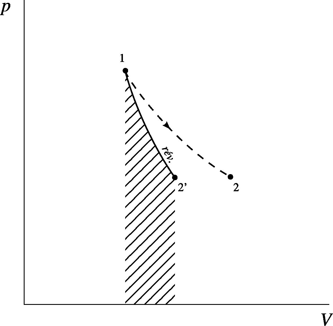
We have seen in chapter 2 (closed systems) that when the process is reversible, the work done by a fluid as its volume changes is expressed by equation 2/14:

W_{\mathrm{A}\rightarrow \mathrm{B}}= -\int _{\mathrm{A}}^{\mathrm{B}} pdV

(8/4)

for a closed system when the volume changes are infinitely slow.

We could thus propose to define volume as being “what varies with pressure when work is done, when the process is reversible”, which would amount to the following definition:

dV = -\left(\frac{\mathrm{δ}W}{p}\right)_{\mathrm{rev}.}

(8/5)

where the subscript rev. indicates the calculation is done along a reversible path.

or even the following, more approachable expression, which can be visualized on a pressure-volume diagram (figure 8.2):

\Delta V = -\int _{\mathrm{A}}^{\mathrm{B}} \left(\frac{\mathrm{δ}W}{p}\right)_{\mathrm{rev}.}

(8/6)

where the subscript rev. indicates the calculation is done along a reversible path.

We can see that entropy is defined in a similar way, that is, as the variable $S$ that, during a reversible heat transfer, allows us to relate heat to temperature with the relation 8/2:

\Delta S = \int _{\mathrm{A}}^{\mathrm{B}} \left(\frac{\mathrm{δ}Q}{T}\right)_{\mathrm{rev}.}

(1)

where the subscript rev. indicates the calculation is done along a reversible path.

Volume changes during adiabatic expansions. The increase in volume is calculable by integrating $\delta W/p$ along a reversible path $(1 \rightarrow 2^{'})$, but not along an irreversible path $(1 \rightarrow 2)$. — Figure 8.2:Volume changes during adiabatic expansions. The increase in volume is calculable by integrating $\delta W/p$ along a reversible path $(1 \rightarrow 2^{'})$ , but not along an irreversible path $(1 \rightarrow 2)$ .

Diagram CC-0 Olivier Cleynen

Then we have

Q_{\mathrm{A}\rightarrow \mathrm{B}}= \int _{\mathrm{A}}^{\mathrm{B}} (T dS)_{\mathrm{rev}.}

(8/7)

q_{\mathrm{A}\rightarrow \mathrm{B}}= \int _{\mathrm{A}}^{\mathrm{B}} (T ds)_{\mathrm{rev}.}

(8/8)

for any process, where the subscript rev. indicates the calculation is done along a reversible path.

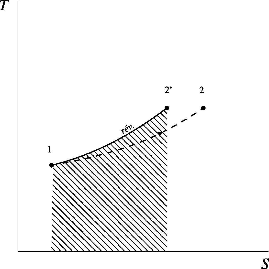
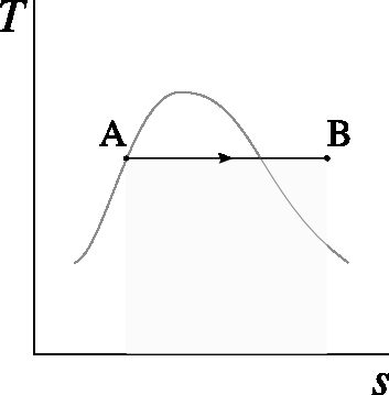
In this way, we are able to represent the processes on a temperature-entropy diagram. As shown in figure 8.3, the area under the curve of a process will represent the heat transferred in cases where the process is reversible; but in cases where the process is irreversible, it does not.

Temperature-entropy diagram. During a reversible process, the area under the curve of a T-s diagram represents the transmitted heat Q_{1→2'}; but not when it is irreversible. — Figure 8.3:Temperature-entropy diagram. During a reversible process, the area under the curve of a $T-s$ diagram represents the transmitted heat $Q_{1\rightarrow 2^{'}}$ ; but not when it is irreversible.

Diagram CC-0 Olivier Cleynen

8.3.2 Temperature-entropy diagrams¶

After six chapters of loyal and dedicated service, the time has come to honorably discharge the pressure-volume diagram, because it is time to make use of our new tool: the temperature-entropy diagram. Even though it is a bit more abstract, the $T-s$ diagram is very useful for describing what happens inside machines because it is easy to plot and allows us to visualize directly the irreversibility, which is always undesirable for the engineer.

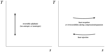
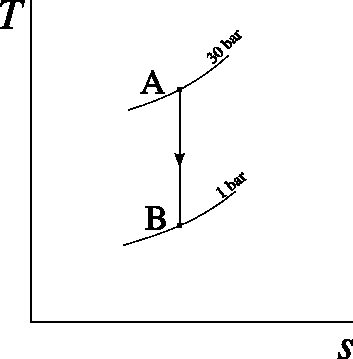
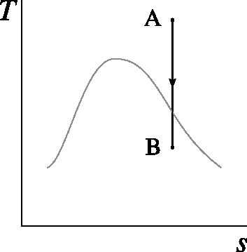
When a fluid receives or supplies work in a reversible adiabatic manner, then $\Delta s = \int \frac{\mathrm{δ}q}{T} = 0$ , since the process is reversible and δ $q = 0$ . A reversible adiabatic process thus occurs at constant entropy – it is iso-entropic, and we call that isentropic. We will represent it as a vertical path on temperature-entropy diagrams (figure 8.4).

Figure 8.4:Elementary processes on temperature-entropy diagrams.

Diagrams CC-0 Olivier Cleynen

Transfer of heat, on the other hand, causes a change in the system’s entropy (positive when heat is received and negative when it is rejected). On $T-s$ diagrams, we move from left to right while receiving heat or when there is irreversibility in a compression or expansion.

When the system loses heat, its entropy decreases and we move from right to left on the $T-s$ diagrams (figure 8.4).

Note also that when a fluid completes a cycle, the temperature at which entropy decreases can be lower than the temperature at which it increases (just like volume with pressure). The net heat transfer is then negative: the fluid has absorbed heat which has been converted into work. If it were to follow the reverse path, the fluid cycle would be a source of heat: this is the operating principle of the refrigerator (§6.2.3).

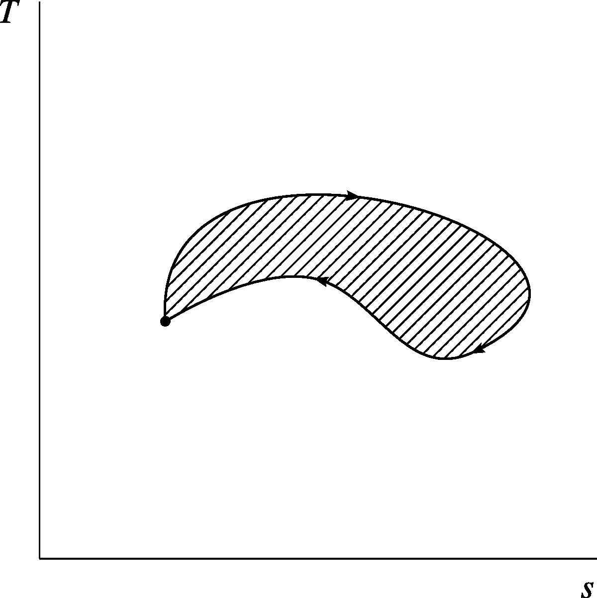
When the processes are reversible, this net heat is represented by the area enclosed by the path taken by the fluid on a temperature-entropy diagram (figure 8.5): a thermodynamic cycle during which heat has been absorbed, and therefore transformed into work; when the path is reversed, heat is rejected (and work absorbed) by the fluid.

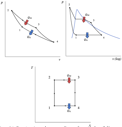
Finally, we are pleased to note that the Carnot cycle, consisting of two isothermal phases $(T =$ constant) separated by two isentropic phases $(s =$ constant), benefits greatly from being represented on a temperature-entropy diagram, as shown in figure 8.6.

Carnot engine cycle, on a 𝑝-𝑣diagram for an ideal gas (left), on a 𝑝-𝑣 diagram for a liquid-vapor system (right), and on a 𝑇-𝑠diagram (bottom). Regardless of the fluid used, the temperature-entropy diagram remains the same. — Figure 8.6:Carnot engine cycle, on a $p-v$ diagram for an ideal gas (left), on a $p-v$ diagram for a liquid-vapor system (right), and on a $T-s$ diagram (bottom). Regardless of the fluid used, the temperature-entropy diagram remains the same.

Diagrams 1, 2 and 3 CC-0 Olivier Cleynen

8.3.3 Entropy changes of an ideal gas¶

From now on, we wish to quantify the entropy change in fluids for any arbitrary process. For an ideal gas, the quantification of this change is surprisingly simple.

For any process undergone by a fixed quantity of fluid, we have (2/2):

q_{1\rightarrow 2}+ w_{1\rightarrow 2}= \Delta u

(2)

If we imagine a reversible path between 1 and 2, we can quantify $q_{1\rightarrow 2}= \int_{1}^{2} T\, ds$ (equation 8/8) and $w_{1\rightarrow 2}= -\int_{1}^{2} p\, dv$ (equation 2/15) along it, and we can write:

\int_{1}^{2} T\, ds - \int_{1}^{2} p\, dv = \Delta u

(3)

T\, ds - p\, dv = du

(8/9)

ds = \frac{du}{T} + \frac{p}{T}\, dv

(4)

during any reversible process.^[1]

Now, if we use an ideal gas, we have $u = c_{v}T$ (equation 4/11) and $p = \frac{RT}{v}$ (equation 4/1), thus:

ds = c_{v}\frac{dT}{T} + R\frac{dv}{v}

(5)

\Delta s = s_{2}- s_{1}= c_{v}\ln \frac{T_{2}}{T_{1}} + R\ln \frac{v_{2}}{v_{1}}

(8/10)

\Delta s = s_{2}- s_{1}= c_{p}\ln \frac{T_{2}}{T_{1}} - R\ln \frac{p_{2}}{p_{1}}

(8/11)

for an ideal gas, for any process from 1 to 2, reversible or not.

This equation is interesting because it indicates that the entropy change $\Delta s$ during a process from 1 to 2 depends only on the initial and final states. Even though we started this demonstration along a reversible process, we obtain an expression 8/10 in which the path used does not appear.

It is therefore possible to easily calculate the change entropy of an ideal gas if its other properties are known. Unlike the internal energy $u$ which depends only on temperature, changes in entropy $(\Delta s)$ also depend on the gas pressure.

In the case where pressure or specific volume is kept constant, these equations 8/10 and 8/11 become respectively:

\Delta s_{v_{\mathrm{const}.}}= c_{v}\ln \frac{T_{2}}{T_{1}}

(8/12)

\Delta s_{p_{\mathrm{const}.}}= c_{p}\ln \frac{T_{2}}{T_{1}}

(8/13)

for an ideal gas, for any process at constant volume or respectively at constant pressure.

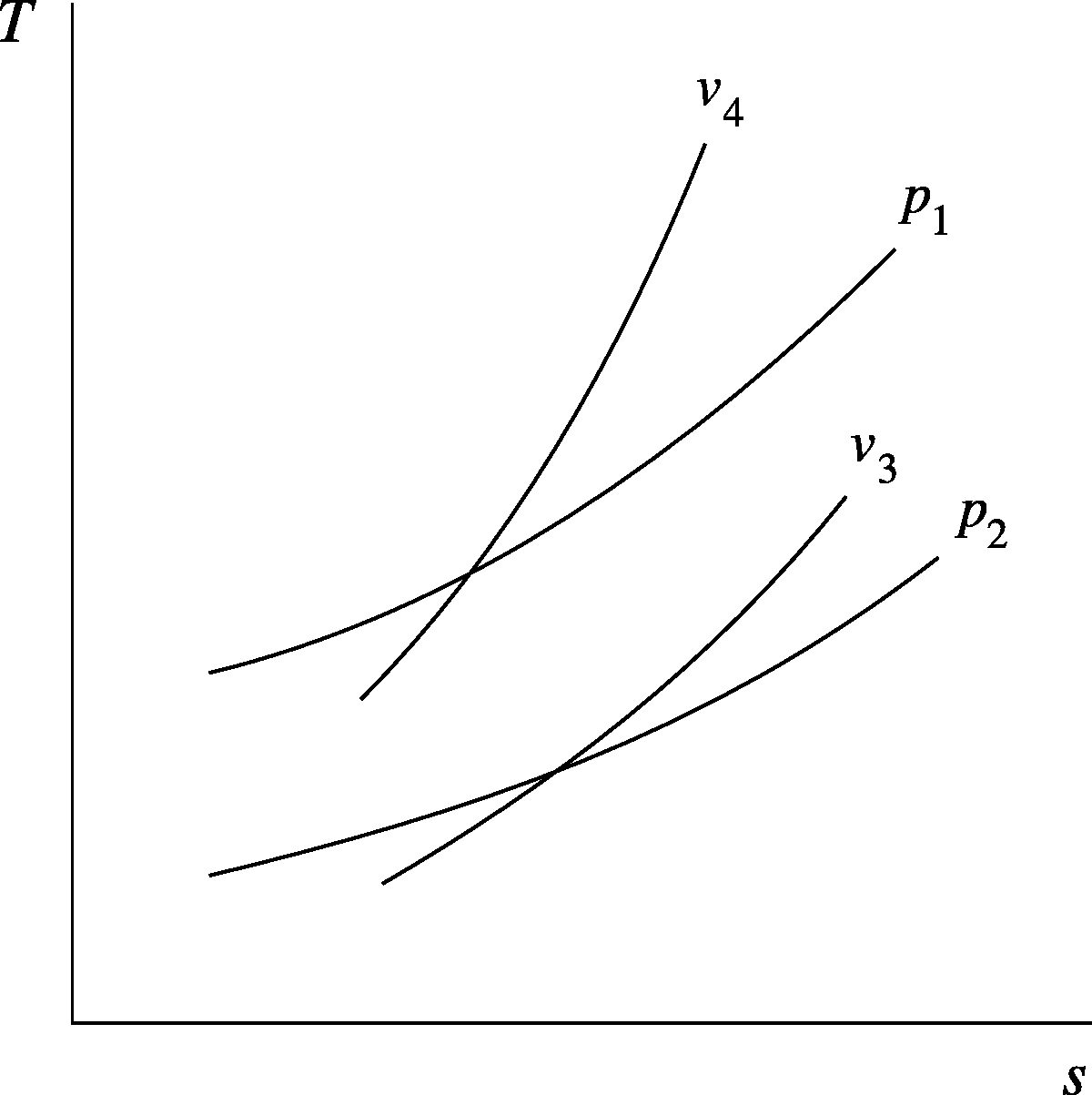
These two equations 8/12 and 8/13 allow us to plot isochoric (at constant volume) and isobaric (at constant pressure) curves for an ideal gas on a $T-s$ diagram, as shown in figure 8.7.

Example 8.2

What is the change in specific entropy of a mass of $2\,\mathrm{kg}$ of air, when it is heated at constant pressure of $2\,\mathrm{bar}$ , from $10^{\circ}\mathrm{C}$ to $100^{\circ}\mathrm{C}$ ?

In order to calculate $\Delta S$ , we start from equation 8/11, $\Delta s= c_{p}\ln\frac{T_{B}}{T_{A}} - R\ln\frac{p_{B}}{p_{A}}$ and here $p_{B}= p_{A}$ . We thus have $\Delta s= c_{p}\ln\frac{T_{B}}{T_{A}}= 1005\ln\frac{100+273.15}{10+273.15}= +277.4\,\mathrm{J\,K^{-1}\,kg^{-1}}$ . The change in entropy is $\Delta S= m\Delta s= 2\times 277.4= +554.8\,\mathrm{J\,K^{-1}}$ .

Isobaric and isochoric curves on a 𝑇-𝑠diagram, for an ideal gas. Here 𝑝1 > 𝑝2 and 𝑣3 > 𝑣4. — Figure 8.7:Isobaric and isochoric curves on a $T-s$ diagram, for an ideal gas. Here $p_{1}> p_{2}$ and $v_{3}> v_{4}$ .

Diagram CC-0 Olivier Cleynen

Example 8.2

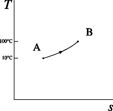
What is the change in specific entropy of a mass of $2 kg (4.4 lb)$ of air, when it is heated at constant pressure of 2 bar, from $50 ^{\circ} F$ to $212 ^{\circ} F (10^{\circ}C$

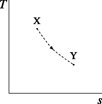
The process can be drawn qualitatively (that is, without showing numerical values) on a temperature-entropy diagram as shown below.

In order to calculate $\Delta S$ , we start from equation 8/11, $\Delta s = c_{p}\ln \frac{T_{\mathrm{B}}}{T_{\mathrm{A}}} - = p_{\mathrm{A}}$ . We thus have $\Delta s = c_{p}\ln \frac{T_{\mathrm{B}}}{T_{\mathrm{A}}} =$

$_{10+273,15}= +277.4 J K^{-1}kg^{-1}$ .

The change in entropy is $\Delta S = m \Delta s = 2 \times 277.4 = +554.8 J K^{-1}$ .

It does not matter whether the process is reversible or not: we just need to know the initial and final states.

We correctly state that “the entropy of the air increases” and not that “entropy is given to it” (§8.2.1).

Example 1

In order to quantify $\Delta S$ we start from equation 8/11, $\Delta s = c_{p}\ln \frac{T_{B}}{T_{A}} - Rln \frac{p_{B}}{p_{A}}$ and here $T_{B}= T_{A}$ . We thus have $\Delta s = -Rln \frac{p_{B}}{p_{A}} = 287 \ln \frac{5}{1} = -461.9 J K^{-1}kg^{-1}$ . The change in entropy is $\Delta S = m \Delta s = 0.5 \times -461.9 = -231 J K^{-1}$ .

Since the process is reversible, the heat removed is obtained using equation 8/7: $Q_{\mathrm{A}\rightarrow \mathrm{B}}= \int ^{\mathrm{B}}_{\mathrm{A}}T dS = T_{\mathrm{cst}.}\int ^{\mathrm{B}}_{\mathrm{A}}dS = T_{\mathrm{cst}.}\Delta S = (50 + 273, 15) \times -231 = -74.6 kJ$ .

We already knew how to quantify $Q_{\mathrm{A}\rightarrow \mathrm{B}}$ without using entropy, using equations 4/27 and 4/28.

Example 2

In order to quantify $\Delta S$ we again start from equation 8/11: $\Delta s = c_{p}\ln \frac{T_{\mathrm{B}}}{T_{\mathrm{A}}} - Rln \frac{p_{\mathrm{B}}}{p_{\mathrm{A}}}$ and here $\Delta s = 0$ :

\ln \frac{T_{\mathrm{B}}0}{T_{\mathrm{A}}} == \frac{c_{p}R}{c_{p}} lnln \frac{T_{\mathrm{B}}p_{\mathrm{B}}T_{\mathrm{A}}}{p_{\mathrm{A}}} - Rln \frac{p_{\mathrm{B}}}{p_{\mathrm{A}}}

(6)

\frac{R}{} \frac{\gamma -1}{}

(7)

( ^{\frac{T_{\mathrm{B}}}{T_{\mathrm{A}}}} ) = (\frac{p_{\mathrm{B}}}{p_{\mathrm{A}}})^{cp}= (\frac{p_{\mathrm{B}}}{p_{\mathrm{A}}}) ^{\gamma}

(8)

Here we recognize the dreaded equation 4/37 which we have wielded

\frac{0.4}{}

(9)

in the past: $T_{\mathrm{B}}= 600 \times \frac{1}{30} ^{1.4}= 227 K$ , approximately $-46^{\circ}C$ or $-51 ^{\circ} F$ .

Using the reasoning “adiabatic reversible = isentropic” did not actually bring us anything we did not already know here, as the ideal gas model is already extremely simple and powerful. This will not be the case with liquids/vapors.

8.3.4 Entropy changes of a liquid/vapor mixture¶

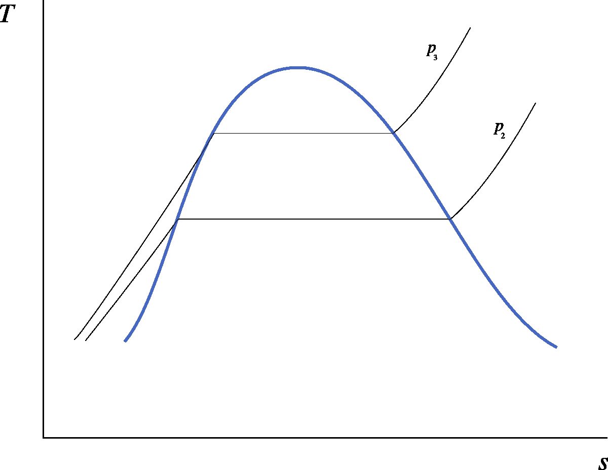
For a liquid/vapor mixture, the changes of $s$ cannot be predicted with a calculation because there is no simple mathematical model to describe temperature as a function of other properties. The saturation curve and the path of process at constant pressure are represented in figure 8.8; this figure closely resembles the temperature-volume diagram we plotted in figure 5.7.

In order to quantify changes in entropy, we we will proceed exactly as we did with internal energy $u$ in chapter 5 (liquids and vapors): by tabulating values for $s$ . Since there is no way to measure $s$ directly, all the tabulated values of entropy are relative to a reference point for which $s$ is arbitrarily set to $0 J K^{-1}kg^{-1}$ ; in our case, it is the triple point of water. This does not matter for our calculations, since we are only interested in the changes of entropy.

Figure 8.8:Temperature-entropy diagram of a liquid/vapor mixture. This figure closely resembles fgi. 5.7 p. 121.

Diagram CC-0 Olivier Cleynen

When water is either in a saturated liquid or dry steam state, values of entropy can simply be read in the last column in Steam Table 1 (see Appendix A1 pp. 306-309, and section §5.3 p. 123), an extract of which is repeated in table 8.1.

Table 8.1:An extract from Steam Table 1 (see pp. 306-309). Values for entropy can be read in the last column, and its values are interpolated like the other properties.

°C $T$	$m^{3}$ $kg$ $v$	$kJ$ $kJ$ $kg$ $kg$ $u$ $h$	$kJ$ $Kkg$ $s$
		$p = 1.6MPa$
		$(T_{\mathrm{sat}.}= 201.37^{\circ}C)$
10	0.001	42 43.6	0.1509
20	0.001001	83.8 85.4	0.2962
50	0.001011	209.1 210.7	0.7031
100	0.001043	418.6 420.3	1.306
200	0.001156	850.4 852.3	2.3305
300	0.15866	2781.5 3035.4	6.8863
500	0.22029	3120.1 3472.6	7.5409
600	0.24999	3293.9 3693.9	7.81
700	0.2794	3473.5 3920.5	8.0557
800	0.30865	3659.5 4153.3	8.2834
900	0.3378	3852.1 4392.6	8.4965
1000	0.36687	4051.2 4638.2	8.6974
1100	0.39589	4256.6 4890	8.8878
1200	0.42487	4467.9 5147.7	9.0689
1500	0.51169	5133.7 5952.4	9.5656
2000	0.65615	6326.8 7376.6	10.272

Within the saturation curve, in other words, when a mix of phases is present, we interpolate values for entropy between those of $s_{L}$ (saturated liquid) and $s_{V}$ (saturated vapor) using the concept of dryness fraction, exactly as with equation 5/5:

s_{x}= s_{L}+ x s_{LV}

(8/14)

Example 8.5

How much does the entropy of water change when it goes from a state at $240^{\circ}C$ and 6 bar, to $130^{\circ}C$ with an internal energy of $1000 kJ kg^{-1}$ ?

A quick look at the steam tables allows us to draw the process qualitatively on a temperature-entropy diagram as shown below. We read $s_{\mathrm{A}}$ by interpolation in Steam Table 1 at $0.6 MPa$ between $200^{\circ}C$ and $300^{\circ}C$ : $s_{\mathrm{A}}= 6.9683 + ^{40}$ Upon arrival, the water is in a liquid-vapor mixture (because $u_{\mathrm{B}}< u_{V130^{\circ}C})$ , so we read from Steam Table 2 (equation 5/5): $x_{\mathrm{B}}= ^{u_{\mathrm{B}}-u_{L}}$

(8/14)

$_{100}\times (7.374 - 6.9683) = 7.1306 kJ K^{-1}kg^{-1}$ .

$u_{LV}= ^{1000-546.1}_{1993.5}=$

Example 5

Since the process is reversible, we can calculate $Q_{\mathrm{A}\rightarrow \mathrm{B}}$ by integrating the term $T ds$ between A and B. We read $s_{\mathrm{A}}$ in Steam Table 2: $s_{\mathrm{A}}= s_{L300^{\circ}C}= 3.2552 kJ kg^{-1}K^{-1}$ . At the end, the specific volume is $v_{\mathrm{B}}= \frac{V_{\mathrm{B}}}{m} = \frac{2}{2} = 1 m^{3}kg^{-1}$ ; in order to obtain $s_{\mathrm{B}}$ we must interpolate between two blocks of Steam Table 1 (between $0.2 MPa$ and $0.4 MPa$ at $300^{\circ}C)$ . Let $y \equiv \frac{v_{\mathrm{B}}-v_{300^{\circ}C \& 0.2 MPa}}{v_{300^{\circ}C \& 0.4 MPa}-v_{300^{\circ}C \& 0.2 MPa}}= \frac{1-1.3162}{0.65489-1.3162}= 0.4781$ and correspondingly, $s_{\mathrm{B}}= s_{300^{\circ}C \& 0.2 MPa}+ y(s_{300^{\circ}C \& 0.4 MPa}- s_{300^{\circ}C \& 0.2 MPa}) = 7.8941 +0.4781(7.5677 - 7.8941) = 7.738 kJ K^{-1}kg^{-1}$ .

Example 7

Here $q_{\mathrm{A}\rightarrow \mathrm{B}}= 0$ because the turbine is adiabatic, and we are looking for $w_{\mathrm{A}\rightarrow \mathrm{B}}= \Delta h$ . Therefore, we need to find a way to quantify $h_{\mathrm{B}}$ .

In A, we read from Steam Table 1, at $4 MPa$ : $h_{\mathrm{A}}= 3446 kJ kg^{-1}$ and $s_{\mathrm{A}}= 7.0922 kJ K^{-1}kg^{-1}$ .

At B, we know that $s_{\mathrm{B}}= s_{\mathrm{A}}$ because the process is isentropic; this information will allow us to calculate $h_{\mathrm{B}}$ . Using Steam Table 3 at $0.05 MPa$ , with equation 8/14, we obtain $x_{\mathrm{B}}= \frac{s_{\mathrm{B}}-s_{L}}{s_{LV}} = \frac{7.0922-1.0912}{6.5018}= 0.923$ . Using the dryness fraction, we can simply calculate the enthalpy (equation 5/4): $h_{\mathrm{B}}= h_{L}+ x_{\mathrm{B}}h_{LV}= 340.5 + 0.923 \times 2304.7 = 2467.7 kJ kg^{-1}$ .

The specific power of the turbine is therefore $w_{\mathrm{A}\rightarrow \mathrm{B}}= \Delta h = -978.3 kJ kg^{-1}$ .

The calculation we have just carried out is extremely useful for engineers. The idea that entropy remains constant during a reversible adiabatic process allows us – at last! – to predict the state of a liquid-vapor mixture at the outlet of a compressor or turbine. Until now, this could be done with an ideal gas (and the cumbersome relationships like $\frac{T_{1}}{T_{2}} =...)$ , but not for a liquid/vapor mixture.

8.4 Predicting the Direction of Processes¶

Here we come to the central concept that has opened the doors of physics to thermodynamics. Based on the quantifications of entropy changes, we are able to describe the direction of processes, that is, to prove for example that a state B comes after a state A.

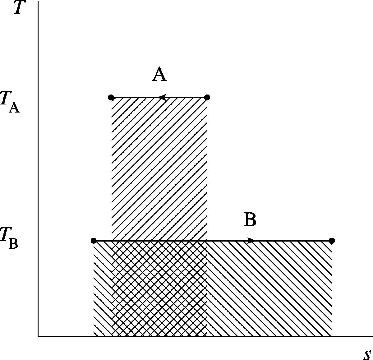
8.4.1 Irreversibilities during heat transfers¶

In order to reward ourselves for already making it halfway through the chapter, we make ourselves a cup of tea. Because no one can resist a little thermodynamics, we press our mug closely against a bottle of cold water. O wonder, o joy! We have before our eyes a source of entropy. Let’s investigate. Our mug A is at temperature $T_{\mathrm{A}}$ , higher than $T_{\mathrm{B}}$ , the temperature of the water bottle (figure 8.9). The two bodies are brought into contact, and an infinitesimal amount of heat $\delta q$ passes from A to B.

If we consider only a small amount of time, the temperature of body A is uniform, and its heat loss occurs reversibly. Thus, the entropy change of A is:

ds_{\mathrm{A}}= -\frac{\delta q}{T_{\mathrm{A}}}

(10)

The temperature of body B is also uniform: the process there is also internally reversible, and the change of its entropy is:

ds_{\mathrm{B}}= +\frac{\delta q}{T_{\mathrm{B}}}

(11)

However, the temperature of the entire system [A+B] is not uniform at all: the process there is not internally reversible. Even if the system receives no heat from the external surroundings, it does not have “a” temperature, and we cannot apply integral 8/2, $\int ^{2}_{1}(T ds)_{\mathrm{rev}.}$ to calculate its entropy change. The entropy change of system [A+B] is the sum of those of its components, namely:

ds_{[\mathrm{A}\&\mathrm{B}]}= ds_{\mathrm{A}}+ ds_{\mathrm{B}}= \frac{\delta q}{T_{\mathrm{B}}} - \frac{\delta q}{T_{\mathrm{A}}}

(8/15)

Figure 8.9:Creation of entropy by heat transfer. The process is internally reversible for each of the two bodies A and B, but irreversible for the system [A+B].

Diagram CC-0 Olivier Cleynen

Since $T_{\mathrm{A}}> T_{\mathrm{B}}$ , this change is positive and non-zero; entropy has been created during the irreversible heat transfer. The irreversibility occurs neither in cup A nor in bottle B, but at the thin material boundary separating them. The process can be represented rather convincingly on a $T-s$ diagram (figure 8.10).

Entropy changes for bodies A and B. The two shaded areas are equal (representing the heat quantity δ$q)$, but the sum of the two entropies increases. — Figure 8.10:Entropy changes for bodies A and B. The two shaded areas are equal (representing the heat quantity δ $q)$ , but the sum of the two entropies increases.

Diagram CC-0 Olivier Cleynen

This small investigation shows us that every temperature gradient leads to irreversibility, resulting in an increase in total entropy. Any heat transfer between two objects of different temperatures can be viewed as a missed opportunity to do work – likely a source of anxiety for both students and engineers. By placing a Carnot engine between bodies A and B, no irreversibility would occur, and $ds_{[\mathrm{A}\&\mathrm{B}]}$ would be zero. By placing a thermal engine with low efficiency, $ds_{[\mathrm{A}\&\mathrm{B}]}$ would be small; the case above where heat transfer occurs without a machine is the limiting case where no work is produced.

8.4.2 Irreversibilities during adiabatic¶

compressions and expansions¶

Another type of process leads to irreversibilities, and thus to an increase in total entropy: it is the transfer of work in fluids.

In practice, any expansion or compression occurs in the presence of internal irreversibilities. Since the duration of the process is finite (unlike Carnot’s idealized processes), there will necessarily be pressure imbalances within the fluid. These imbalances lead to internal turbulence, which causes the conversion of mechanical energy into internal energy through friction and heat.

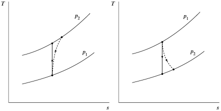
Thus, a real adiabatic compression causes the fluid to reach a higher temperature than a reversible adiabatic compression (figure 8.11): part of the supplied work is completely converted into heat due to internal friction. Accordingly, during a real adiabatic expansion, the temperature decreases less than during a reversible adiabatic expansion. Each time, entropy is increased even though no heat transfer δ $q$ has occurred.

Theoretical (isentropic, solid lines) and real (dotted lines) adiabatic expansions and compressions. It is important to note that the increase in entropy is not related to a heat transfer “δ$q$”. The path on the $T-s$diagram is not continuous, and the area underneath does not represent a heat flow across the system boundaries. — Figure 8.11:Theoretical (isentropic, solid lines) and real (dotted lines) adiabatic expansions and compressions. It is important to note that the increase in entropy is not related to a heat transfer “δ $q$ ”. The path on the $T-s$ diagram is not continuous, and the area underneath does not represent a heat flow across the system boundaries.

Diagrams CC-0 Olivier Cleynen

8.4.3 The second law and entropy¶

We have stated in chapter 7 (the second law) that heat spontaneously moves only towards a lower temperature – a postulate we call the second law. We can now formulate this statement with a mathematical expression.

During a heat transfer from a body at temperature $T_{\mathrm{A}}$ to another at temperature $T_{\mathrm{B}}$ , the overall entropy change $\Delta s = \frac{-q}{T_{\mathrm{A}}} + \frac{q}{T_{\mathrm{B}}}$ is necessarily zero or positive because $T_{\mathrm{A}}$ is necessarily equal to or greater than $T_{\mathrm{B}}$ .

During a work transfer any irreversibility results in a higher final temperature than it could have been (see §2.4.3). Achieving the same final state with a reversible path thus requires a heat input, in other words, a positive term $\int (\frac{\mathrm{δ}Q}{T})_{\mathrm{rev}.}$ . An irreversibility therefore leads to an increase in total entropy.

Thus, we can translate the second law as follows:

When an energetically-isolated system undergoes a process, its entropy $s$ changes in such a way that

\Delta s \geq 0

(8/16)

We can always decrease the entropy of a system to bring it back to its initial value (by returning the system itself to its initial state, whatever the method used), but this will necessarily be at the expense of an increase at least as large in the entropy of another system.

We could also say, in the same way that we described energy as “a quantity that does not change during transformations” (§1.1.1), that entropy is conceptualized as “a quantity that always increases during transformations.” This is the indicator we were looking for in §8.1.1 to determine the direction of processes.

8.4.4 Predicting the direction of processes¶

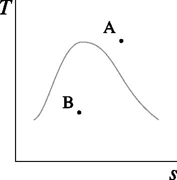
In order to demonstrate that a system can only go from state A to state B, in other words, that the process is irreversible, we need to proceed as follows:

We need to find a reversible path A $\rightarrow$ B, namely, a process to go from A to B while keeping pressure and temperature internally homogeneous even if they vary;
Along this reversible path, we calculate $\Delta s$ (that is, we carry out the integral $\int \frac{\mathrm{δ}q}{T}$ for this path).
We compare the integral $\int \frac{\mathrm{δ}q}{T}$ along the reversible path with the integral for the real path.

There are three possibilities:

• If the two integrals are equal, then the real process is reversible: it can take place in both directions.

• If $\int (\frac{\mathrm{δ}q}{T})_{\mathrm{real} \mathrm{path}}< \int (\frac{\mathrm{δ}q}{T})_{\mathrm{rev}.}$ , then the real process is irreversible. It can only take place from A to B.

• If $\int (\frac{\mathrm{δ}q}{T})_{\mathrm{real} \mathrm{path}}> \int (\frac{\mathrm{δ}q}{T})_{\mathrm{rev}.}$ , then the described “real” process is

impossible. It can only take place in the reverse direction (B $\rightarrow$ A).

Thus, we can mathematically determine the direction of time, at least for some simple cases – a subtlety that one would not expect from engineers concerned about their fuel consumption!

Example 8.8

A mass of air undergoes a process without any heat exchange. There are two states:

• State X at 5 bar and $100^{\circ}C (72.5 psi$ and $212 ^{\circ} F)$ ;

• State Y at 1 bar and $5^{\circ}C (14.5 psi$ and $41 ^{\circ} F)$ .

In which direction (X $\rightarrow$ Y or Y $\rightarrow$ X) can the process take place?

Let’s suggest the direction X $\rightarrow$ Y and check if it is physically possible.

The entropy change is equal to the integral $\int _{\mathrm{X}}^{\mathrm{Y}}\left(\frac{\delta q}{T}\right)_{\mathrm{rev}.}$ . Using equation 8/11, $\Delta s= c_{p}\ln\frac{T_{\mathrm{Y}}}{T_{\mathrm{X}}} - R\ln\frac{p_{\mathrm{Y}}}{p_{\mathrm{X}}}= 1005\ln\frac{5+273.15}{100+273.15} - 286\ln\frac{1}{5}= +166.6\,\mathrm{J\,K^{-1}\,kg^{-1}}$ .

On the other hand, the integral $\int _{\mathrm{X}}^{\mathrm{Y}}\left(\frac{\delta q}{T}\right)_{\mathrm{real}\,\mathrm{path}}$ is equal to zero because in reality there was no heat transfer ( $\delta q= 0$ ).

Therefore, we have $\Delta s > \int _{\mathrm{X}}^{\mathrm{Y}}\left(\frac{\delta q}{T}\right)_{\mathrm{real}\,\mathrm{path}}$ and the process is irreversible. If we wanted to reverse the process, from Y to X, we would have to remove heat.

diagram as follows:

Example 8.9

Water undergoes a process during which $1 MJ kg^{-1}$ of heat is added to it at while its temperature is fixed at $130^{\circ}C (266 ^{\circ} F)$ . There are two states, one at the beginning and the other at the end:

• State X as liquid at $130^{\circ}C$ and saturated;

• State Y as vapor at $170^{\circ}C (338 ^{\circ} F)$ and saturated.

In which direction (X $\rightarrow$ Y or Y $\rightarrow$ X) can the process take place?

Let’s consider the direction X $\rightarrow$ Y and verify if it is physically possible.

We read the values of entropy in Steam Table 2: $s_{\mathrm{X}}= s_{L\,130^{\circ}\mathrm{C}}= 1.6346\,\mathrm{kJ\,K^{-1}\,kg^{-1}}$ and $s_{Y}= s_{V\,170^{\circ}\mathrm{C}}= 6.665\,\mathrm{kJ\,K^{-1}\,kg^{-1}}$ . Thus, $\Delta s= \int _{\mathrm{X}}^{\mathrm{Y}}\left(\frac{\delta q}{T}\right)_{\mathrm{rev}.}= +5.03\,\mathrm{kJ\,K^{-1}\,kg^{-1}}$ .

Separately, we can calculate the integral $\int _{\mathrm{X}}^{\mathrm{Y}}\left(\frac{\delta q}{T}\right)_{\mathrm{real}\,\mathrm{path}}$ because we know that heat was supplied when the temperature was fixed at $130^{\circ}\mathrm{C}$ . Thus $\int _{\mathrm{X}}^{\mathrm{Y}}\left(\frac{\delta q}{T}\right)_{\mathrm{real}\,\mathrm{path}}= \frac{1}{T}\int _{\mathrm{X}}^{\mathrm{Y}}(\delta q)_{\mathrm{real}\,\mathrm{path}}= \frac{q_{\mathrm{X}\rightarrow \mathrm{Y}}}{T}= \frac{1\times 10^{6}}{170+273.15}= +2.26\,\mathrm{kJ\,K^{-1}\,kg^{-1}}$ .

The process can be drawn qualitatively on a temperature-entropy diagram as follows:

Here, we have $\Delta s > \int _{\mathrm{X}}^{\mathrm{Y}}(\frac{\mathrm{δ}q}{T})_{\mathrm{real} \mathrm{path}}$ and the process is irreversible. If we wanted to go back from Y to X, we would need to cool the water by removing a quantity necessarily greater than $1 MJ kg^{-1}$ .

8.5 Entropy, Time, and the Universe¶

8.5.1 Entropy for the engineer¶

We have seen that entropy, just like energy, is a concept which was designed in order to back with calculations an intuition that we have about the world: quantifying their changes enables us to determine the transformations that are possible. It is therefore fundamentally a concept for physicists. For engineers, entropy is:

• “what does not change when compressing and expanding fluids ideally”. Thus, quantifying $\Delta s$ allows us to quantify the properties that a fluid should have at the outlet of a compressor or a turbine;

• “what does not change when transferring heat within a system ideally”. Thus, quantifying $\Delta s$ allows us to calculate the irreversibility that occurs during heat transfers.

Whenever we produce an increase in overall entropy, we have to proceed ultimately to an unwanted heat rejection. Thus, these quantifications of $\Delta s$ allow us to measure the quality of expansions, compressions, cooling, and heating that we carry out with fluids in our machines.

8.5.2 Context: the direction of time¶

The examples we have studied in this chapter to determine the direction of processes are very academic, however the approach remains valid for any process: a stone thrown into a pond, a food plate breaking when it falls, etc. If we go back to the three photos in figure 8.1, we could determine their order by finding the initial and final states of the water around the diver, and comparing $\Delta s$ with the integral $\int (\frac{\mathrm{δ}q}{T})_{\mathrm{real} \mathrm{path}}$ carried out during the entry into the water.

This desire to find the absolute order in which states succeed one another, in other words, the direction of time, led the German physicist Rudolf Clausius to propose the concept of entropy in 1865 in a masterly publication — Über verschiedene für die Anwendung bequeme Formen der Hauptgleichungen der mechanischen Wärmetheorie [17, 18, 19]. Concluding a decade of work around the quantity $\frac{Q}{T}$ , he formalized a concept that his French colleague Frédéric Reech and Scottish counterpart William Rankine had only touched upon [36], and synthesized all the contemporary knowledge of his discipline.

Clausius created the word entropy based on the ancient Greek tropè τροπή (revolution, change), which, coupled with his authoritarian tone, did nothing to win the enthusiasm of his contemporaries. But the concept is so powerful, and equation 8/16 so simple, that they were universally accepted.

After a century of efforts, the physics of heat had caught up with engine technology. We were finally able to fully and quantitatively describe the behavior of bodies without having to delve into that of their constituents, such as molecules, atoms, or subatomic particles: entropy was the last missing piece of what we now call macroscopic thermodynamics.

8.5.3 Entropy at the microscopic scale¶

After Clausius, the development of thermodynamics is no longer of great interest to engineers, but physicists may still be longing for more. Indeed, although we had described the irreversibility phenomenon, we had not yet explained its origin within bodies made up of particles whose movements (an incessant buzzing of collisions, based on attractive and repulsive forces), themselves, are perfectly reversible.

It would take only ten years for the answer to be formalized: in 1875, Austrian physicist Ludwig Boltzmann proposed a microscopic definition of entropy:

S \equiv kln \lambda

(8/17)

where $\lambda$ is the number of possible configurations of the system which correspond to its state, and $k$ is a constant.

Thus, for Boltzmann, entropy is a measure of the probability that the system is in the state in which it is observed. The more probable the configuration (homogeneity of pressure and temperature), the greater the entropy.

At the macroscopic scale, we had described the second law as an impossibility (§7.1.1): for example, an object at one temperature cannot spontaneously have one of its ends cool down while the other heats up. According to Boltzmann, such an event is not strictly impossible, but only very improbable. The state where the fastest molecules are all gathered at one end, and the slowest at the other, is much less probable (lower entropy) than a state where they are distributed homogeneously (higher entropy).

This approach not only has the merit of reconnecting our discipline with atomic theory – and hence we will talk about microscopic thermodynamics and statistical thermodynamics – but it also opened the door to information theory. Indeed, the resolution and precision with which we evaluate the state of a system affect the number of possible configurations that can be attributed to it. Here, the concept of information became linked to other physical properties: an impressive result for a discipline that was only intended to explore what “hot” meant!

8.5.4 Entropy and the universe¶

We leave entropy on an open question. To the extent that we think of the universe as a finite set, in other words, as an isolated system containing a fixed amount of energy, can we apply equation 8/16: $\Delta s_{\mathrm{universe}}> 0$ as time passes? Is the universe moving towards a final homogeneous minimum temperature? Clausius was unequivocal: he immediately concluded his 1865 article with the affirmation:

If for the entire universe we conceive the same magnitude to ^{\mathrm{William} \mathrm{Thomson}, 1852 [12]}

(12)

be determined [...] which for a single body I have called entropy, and if at the same time we introduce the other and simpler conception of energy, we may express in the following manner the fundamental laws of the universe which correspond to the two fundamental theorems of the mechanical theory of heat.

The energy of the universe is constant.
The entropy of the universe tends to a maximum.

Rudolf Clausius, 1865 [17, 18, 19]

Is the theory of refrigerators and engines capable of predicting the end of the world? To explore this question in a fun way, students may read The Last Question by Isaac Asimov [29, 32] or Entropy and all that by Philippe Depondt [43]. For a more formal answer, one must refer to a good physics textbook.

A Bit of History

The history of science also includes some rather romantic figures!

Rumford, an Adventurer Who Weighed Heat

By Philippe Depondt

Pierre and Marie Curie University, Paris

He was actually named Benjamin Thompson (1753-1814) and was an American from Woburn, Massachusetts [40]. He initially had many diverse occupations: clerk in a store, teacher, medical student... However, when the American Revolution broke out, New England where he lived was at the heart of the conflict; Thompson chose the Loyalist side and became a secret agent for the British. At the time of the Declaration of Independence of the United States of America in 1776, cautiously, he left for England.

Figure 8.12:Sir Benjamin Thompson of Rumford, militia fighter, secret agent, architect, Minister of War, bold experimenter, cosmopolitan seducer, and of course, thermodynamicist.

Engraving by J. P. P. Rauschmayr, 1797 (public domain)

He then undertook research on projectiles and joined the Royal Society in 1779. He nevertheless returned to America in 1782 still to fight on the British side, but peace was declared the following year. He was ennobled as Baron Rumford by King George iii in reward for his services. He then became an advisor to the Elector of Bavaria, and later the Minister of War. During his 14 years spent in Bavaria, he reformed the army, established assistance for the needy, and created the famous Englischer Garten in Munich. He then returned to England, and finally settled in France in 1805 where he had a –disastrous– marriage with Marie Lavoisier, the widow of the chemist who was guillotined during the French Revolution.

During his adventurous life, he managed to make at least two important discoveries. Within the framework of the caloric theory, he attempted to weigh heat by measuring the weight of bodies at different temperatures. From these unsuccessful attempts, he concluded that heat has no weight. Later, during his tenure as Minister of War, he oversaw the drilling of cannons and observed in 1798 that the drilling process heated the barrels to the point of boiling water. He realized that the amount of heat released was not limited by the quantity of matter containing it. From this, he deduced that the heat was not stored in the material but rather produced by the work of the horses driving the drill—a foreshadowing of Joule’s first law.

Problems¶

The properties of water are tabulated in Steam Tables 1, 2, and 3 (see Appendix A1 p. 305)

Air is considered an ideal gas.

$c_{v (\mathrm{air})}= 718 J kg^{-1}K^{-1} \qquad R_{\mathrm{air}}= 287 J kg^{-1}K^{-1}$

$c_{p (\mathrm{air})}= 1005 J kg^{-1}K^{-1} \qquad \gamma _{\mathrm{air}}= 1.4$

We assume that for a reversible adiabatic process (without heat transfer and infinitely slow), the properties of air are linked according to the following three relationships:

\left(\frac{T_{1}}{T_{2}}\right) = \left(\frac{v_{2}}{v_{1}}\right)^{\gamma -1} \qquad (4/36)

(13)

\left(\frac{T_{1}}{T_{2}}\right) = \left(\frac{p_{1}}{p_{2}}\right)^{\frac{\gamma -1}{\gamma}} \qquad (4/37)

(14)

\left(\frac{p_{1}}{p_{2}}\right) = \left(\frac{v_{2}}{v_{1}}\right)^{\gamma} \qquad (4/38)

(15)

We also assume that the change in entropy of an ideal gas, for any evolution, is quantified by the following relations:

\Delta s = s_{2}- s_{1}= c_{v}\ln \frac{T_{2}}{T_{1}} + R\ln \frac{v_{2}}{v_{1}} \qquad (8/10)

(16)

\Delta s = s_{2}- s_{1}= c_{p}\ln \frac{T_{2}}{T_{1}} - R\ln \frac{p_{2}}{p_{1}} \qquad (8/11)

(17)

Finally, we assume that the efficiencies of thermal machines based on a Carnot cycle are expressed as a function of the absolute temperatures as follows:

\eta _{\mathrm{Carnot\ engine}}= 1 - \frac{T_{L}}{T_{H}} \qquad (7/6)

(18)

\eta _{\mathrm{Carnot\ refrigerator}}= \frac{1}{\dfrac{T_{H}}{T_{L}} - 1} \qquad (7/7)

(19)

\eta _{\mathrm{Carnot\ heat\ pump}}= \frac{1}{1 - \dfrac{T_{L}}{T_{H}}} \qquad (7/8)

(20)

Exercise 8.1

Knowledge Recap Questions In order to tackle problems on such a substantial topic, it is necessary to first master the basics! 1. How is the change in the entropy of a body calculated during any real process? 2. Can the entropy of a body ever be reduced? 3. What is the difference between specific entropy and thermal capacity (both have the same units!)? 4. What would figure 8.10 p. 225 look like if the heat transfer was continued beyond an infinitesimal amount of heat δ $Q$ until the mug A and the water bottle B were at the same temperature?

Answer

See §8.2.2 page 211; 2) Yes, a simple heat extraction is enough: see example 8.1 page 211; 3) Specific thermal capacity: heat per unit mass δ $q$ needed to generate a temperature change $dT$ (equation 1/16 page 21: $c \equiv \frac{\mathrm{δ}q}{dT}$ ). Specific entropy: specific heat divided by the temperature at which it issuppliedduring a reversible process(equation8/2 page 211); 4) Both temperatures change until they equalize; $\Delta s_{\mathrm{A}}+ \Delta s_{\mathrm{B}}> 0$ .

Figure 8.13:Reversible elementary processes of an ideal gas, represented on a temperature-entropy diagram.

Exercise 8.3

Expansion of a Liquid/Vapor We have $10 kg (22 lb)$ of water at $45 bar$ and $600^{\circ}C$ $(653 psi$ and $1112^{\circ} F)$ . 1. What is the maximum amount of work that can be extracted from this mass of water without supplying heat, if it can expand to $4 bar (58 psi)$ ? 2. If the expansion were continued to a lower pressure, at what temperature would the water condense? 3. Draw the process qualitatively (that is, without showing numerical values) on a temperature-entropy diagram, showing the saturation curve.

Answer

$u_{1}= 3276.4 kJ kg^{-1}$ and $u_{2}= 2703.3 kJ kg^{-1}$ : $W_{\max.}= -5.731 MJ$ ;
$T_{3}= 103.51^{\circ}C = 218.32 ^{\circ} F$ .

Exercise 8.6

Carnot Cycle Draw the cycle undergone by the fluid inside a heat pump operating according to the Carnot cycle on a temperature-entropy diagram, qualitatively, showing also the two heat transfers. How would the cycle be modified if the compression and expansion remained adiabatic but were not reversible? How would the two heat transfers be affected?

Answer

In this case $W_{\mathrm{B}\rightarrow \mathrm{C\ irr}.}> W_{\mathrm{B}\rightarrow \mathrm{C}'}$ and, as negative values, $W_{\mathrm{D}\rightarrow \mathrm{A\ irr}.}> W_{\mathrm{D}\rightarrow \mathrm{A}'}$ . Thus the rejected heat $Q_{\mathrm{C}\rightarrow \mathrm{D}}$ increases (which may initially seem like an interesting result) and the heat intake $Q_{\mathrm{A}\rightarrow \mathrm{B}}$ decreases (and we see that the increase in $Q_{\mathrm{C}\rightarrow \mathrm{D}}$ is actually only due to the inefficiencies of the compressor and the turbine and only serves to reduce the efficiency).

Exercise 8.7

Steam Turbine In the engine room of a large ship (figure 8.14), a steam flow rate of $250 t/h (\sim 550 000 lb/h)$ enters the turbine at 55 bar and $660^{\circ}C (798 psi$ and $1220 ^{\circ} F)$ . Photo CC-by-sa by Tony Kent

Figure 8.14:Inspection window of one of the low-pressure turbines (power approximately $25 MW)$ of the aircraft carrier USS Hornet launched in 1943.

In the turbine, steam expands following an approximately reversible adiabatic process. When the pressure reaches 1 bar, steam is extracted at a low flow rate $(1 kg s^{-1})$ to heat another part of the power plant. The remaining steam in the turbine is expanded to a pressure of $0.18 bar (2.6 psi)$ . What is the power delivered by the turbine?

Answer

The process is as described in example 8.7 page 223: $h_{1}= 3803.5 kJ kg^{-1}$ (dry steam); $h_{2}= 2677.7 kJ kg^{-1}$ (dry steam); $h_{3}= 2413.6 kJ kg^{-1}$ (mixture with 91.9% dryness fraction); thus $\dot{W}_{\mathrm{turbine}}= -96.26 MW$ .

Exercise 8.8

Direction of Processes (1) A mass of air undergoes a process without any heat transfer. There are two states: • State X: at 1 bar and $300^{\circ}C$ ; • State Y: at 5 bar and $500^{\circ}C$ . In which direction (X $\rightarrow$ Y or Y $\rightarrow$ X) can the process take place? Draw the process on a pressure-volume diagram and on a temperature-entropy diagram, qualitatively.

Answer

With equation 8/11 we find $s_{\mathrm{Y}}- s_{\mathrm{X}}= -161.08 J K^{-1}kg^{-1}< \int _{\mathrm{X}}^{\mathrm{Y}}\left(\frac{\delta q}{T}\right)_{\mathrm{real\ path}}= 0 kJ K^{-1}kg^{-1}$ (since the process is adiabatic). Therefore, the direction is Y $\rightarrow$ X.

Exercise 8.9

Direction of Processes (2) Water undergoes a process during which $2 MJ kg^{-1}$ of heat is extracted from it, while its temperature is fixed at $250^{\circ}C$ . There are two states, one at the beginning and the other at the end: • State X: in the saturated vapor state at $200^{\circ}C$ ; • State Y: in the saturated liquid state at $240^{\circ}C$ . Which of the two states must have occurred before the other?

Answer

Assuming X $\rightarrow$ Y, then $\Delta s = -3.728 kJ K^{-1}kg^{-1}$ but $\int _{\mathrm{X}}^{\mathrm{Y}}\left(\frac{\delta q}{T}\right)_{\mathrm{real\ path}}= -3.823 kJ K^{-1}kg^{-1}$ , so we are reassured: the direction is indeed X $\rightarrow$ Y.

Exercise 8.10

Expansion of Compressed Air The air in a thermally insulated cylinder is expanded from $6.8 bar$ and $430^{\circ}C$ to $1 bar$ . At the end of the expansion, the temperature is measured at $150^{\circ}C$ . Is the expansion reversible? Draw the process qualitatively on a temperature-entropy diagram.

Answer

With equation 8/11 we get $\Delta s = +39.77 J K^{-1}kg^{-1}$ but – aha! – $\int _{1}^{2}\left(\frac{\delta q}{T}\right)_{\mathrm{real\ path}}= 0 kJ K^{-1}kg^{-1}$ , thus the process is irreversible. We could also have used the very classic equation 4/37 p. 103 to find that $T_{2 \mathrm{isentropic}}< 150^{\circ}C$ .

Exercise 8.11

Air Pump Air enters a small centrifugal pump with a flow rate of $4 kg/\min$ (figure 8.15). The pump is not isentropic, but its heat losses can be neglected. At the inlet, the air is at 1 bar and $15^{\circ}C$ . At the outlet, the pressure is 2 bar and the temperature is measured at $97^{\circ}C$ . 1. What is the power required to operate the compressor? 2. What would be the power if the compression were isentropic? Photo CC-by-sa Jakob Voß (cropped) 3. What would be the heat and work transfers required to return the air to its initial conditions (minimizing heat transfers)?

Answer

$1)\dot{W}_{\mathrm{pump}}=\dot{mc}_{p}\Delta T = +5.493 kW$ (equations 3/15 & 4/13); 2) Using equation 4/37 $T_{2\mathrm{is}.}= 351.3 K$ , that is, $78.1^{\circ}C$ or $172.7 ^{\circ} F$ , thus $\dot{W}_{\mathrm{ideal}}= +4.231 kW$ ; 3) One possibility: isentropic expansion to obtain $W_{2\rightarrow 1}= -4.231 kW$ , then a necessary cooling without work of $\dot{Q}_{2\rightarrow 1}= -1.262 kW$ . All reversible processes with a net sum of transfers taking these values(for example during a cooled expansion)will allow to return to 1.

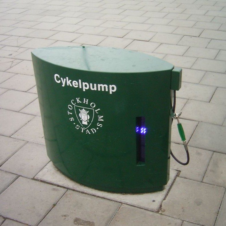
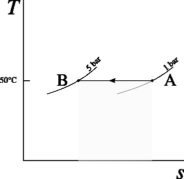
Figure 8.15:Public air compressor in Stockholm for cyclists. A heat exchanger integrated under the bodywork fortunately ensures the temperatures calculated in this problem are never attained.

Exercise 8.12

Theoretical Power Plant During the design of an power plant, a group of enthusiastic engineers is studying the possibility of having water follow a Carnot cycle. The heat released by coal combustion is transferred to a steam boiler. The steam is expanded in a turbine, which powers an electric generator. From A to B Water is compressed in an isentropic pump. At A, the liquid-vapor mixture is at a pressure of $0.04 bar (0.58 psi)$ . At B, the water is in the saturated liquid state, at a pressure of $40 bar (580 psi)$ . From B to C Water is heated at constant pressure $(40 bar)$ in the boiler. At C, the water is in the saturated vapor state. From C to D Water is expanded in an isentropic turbine. At D, the water is at the initial pressure, that is, 0.04 bar. From D to A Water is cooled in a condenser at constant pressure $(0.04 b$ ar). 1. Sketch the elements of the circuit followed by the steam, and draw the process qualitatively on a temperature-entropy diagram, showing the saturation curve. 2. What is the dryness fraction of the water when condensation is interrupted (at A)? What is the specific enthalpy at that point? 3. What is the dryness fraction at the turbine outlet (at D) and the specific enthalpy at this point? 4. What is the power delivered by the turbine? 5. What is the power of the boiler? 6. What is the power of the pump? 7. What is the efficiency of the power plant?

Answer

The diagram is presented in figure 7.17 p. 202; $2) x_{\mathrm{A}}= \frac{s_{\mathrm{B}}-s_{L}}{s_{LV}} = 0.2949; \mathrm{thus} h_{\mathrm{A}}= h_{L}+ x_{\mathrm{A}}h_{LV}= 838.7 kJ kg^{-1}$ ; 3) Same process: $x_{\mathrm{D}}= 0.7014$ thus $h_{\mathrm{D}}= 1827.5 kJ kg^{-1}$ ; 4) $w_{\mathrm{turbine}}= h_{\mathrm{D}}- h_{\mathrm{C}}= -973.3 kJ kg^{-1}$ ; 5) $q_{\mathrm{boiler}}= h_{\mathrm{C}}- h_{\mathrm{B}}= +1713 kJ kg^{-1}$ ; 6) $w_{\mathrm{pump}}= h_{\mathrm{B}}- h_{\mathrm{A}}= +248.8 kJ kg^{-1}$ ; 7) $\eta _{\mathrm{plant}}= \left|\frac{w_{\mathrm{net}}}{q_{\mathrm{in}}}\right| = \frac{-w_{\mathrm{turbine}}-w_{\mathrm{pump}}}{q_{\mathrm{boiler}}} = 42.29\%$ . Since all phases are reversible and heat transfers are isothermal, we have $\eta _{\mathrm{plant}}= \eta _{\mathrm{Carnot\ engine}}= 1 - \frac{T_{\mathrm{condenser\ water}}}{T_{\mathrm{boiler\ water}}}$ (7/6).

Exercise 8.13

Irreversible Heat Transfers A steam engine operates on a Carnot cycle, with a steady flow rate of $2 kg s^{-1}$ , between the saturation points of water. The engine is designed to exploit a heat source at a moderate temperature $(300^{\circ}C)$ , from the combustion of industrial waste, and it rejects heat into a river at a low temperature $(5^{\circ}C)$ . The boiler has thick walls to reduce the impact of manufacturing imperfections and to withstand the high pressure of the water. This thickness imposes a significant temperaturegradientacrossthewalls,addingupto $10^{\circ}C$ . The same applies to the condenser (also $10^{\circ}C$ across the walls). 1. What is the rate of increase of entropy of the {heat source + water} system? 2. What is the rate of increase of entropy of the {heat sink + water} system? 3. What is the power loss associated with this increase in entropy? 4. Which physical properties of the boiler wall material are most desirable to minimize this issue?

Answer

$1)\dot{S}_{\mathrm{high} \mathrm{temp}. \mathrm{wall}}=\dot{m} (\Delta s_{\mathrm{combustion}}+ \Delta s_{\mathrm{water}}) = +91.77 J/(K s) = +91.77 W K^{-1}$ ; $2)\dot{S}_{\mathrm{low} \mathrm{temp}. \mathrm{wall}}= +188.3 W K^{-1}$ , and we see that a gradient of $10^{\circ}C$ is more penalizing at low temperature than at high temperature; $3)\dot{W}_{\mathrm{lost}}=\dot{Q}_{i}nn(\eta _{\mathrm{high} \mathrm{temp}.}- \eta _{\mathrm{low} \mathrm{temp}.}) = 77.9 kW$ 4) To reduce temperature gradients, materials with very high thermal conductivity are needed (this is of course not the only quality required of them… ).

Exercise 8.14

Irreversible Compressions and Expansions The team of engineers in charge of the engine from the previous problem (Carnot cycle operating between $290^{\circ}C$ and $15^{\circ}C$ , problem 8.13) discovers that the compression and expansion phases are not reversible. The compressor does bring the water to a high temperature, but its energy consumption is $10 \%$ higher than expected. The turbine does bring the water to a low temperature,butitsupplies $10 \%$ less work than expected. 1. What is the rate of increase of entropy of the steam in each of these two components? 2. By how much do the heat rejections increase? 3. What is the efficiency loss of the system compared to a reversible system?

Answer

$\Delta s_{\mathrm{compressor}}= +67 J K^{-1}kg^{-1}$ ; $\Delta s_{\mathrm{turbine}}= +382 J K^{-1}kg^{-1}$ ;
$\Delta q_{\mathrm{out}}= -110.2 kJ kg^{-1}$ , or $+14.6 \%$ ;
$\eta _{\mathrm{real} \mathrm{plant}}= 39.82 \%$ , or $-9 pt$ .

Footnotes¶

This equation 8/9 is even true for any process, but this generalization is simpler to address after equations 8/10 and 8/11.
↩