3. Open Systems January 1, 2025
3. Open Systems ¶ Open Systems
Measuring the Intangible in the Ungraspable
Introduction ¶ In the previous chapter, we quantified energy exchanges within closed systems. This chapter 3 (open systems ) aims to answer a similar question: how to quantify energy transfers within a system when it is crossed by a mass flow?
3.1 Why Use an Open System? ¶ In many machines, the fluid used to transfer heat and work is continuously circulating. It can then be difficult to identify a particular amount of mass, making it a closed system, in order to quantify energy transfers to and from it. For example, in a jet engine nozzle, air expands and accelerates continuously: at any given moment, there is no identifiable volume that would have one specific speed or one particular pressure.
Using an open system is very useful to account for energy in flows. Rather than separating stages in time (for example before and after compression), we quantify work and heat transfers by separating stages in space (for example upstream and downstream of the compressor).
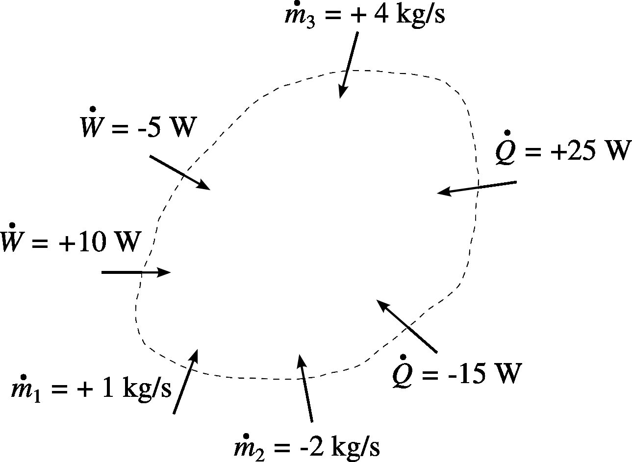
3.2 Accounting Conventions ¶ 3.2.1 The open system ¶ We call an open system an arbitrary subject of study whose boundaries are permeable to mass (figure 3.3). In general, its volume can change, and it can have multiple inlets and outlets, each with a different flow rate and pressure.
Figure 3.1: Sign conventions for an open system. Inflows are positive, outflows are negative; they are all represented with inward arrows.
In our study of thermodynamics, we will only use open systems:
• with fixed volume;
• having only one inlet and one outlet;
« The constructive difficulties that have to be overcome in a large gas motor because of the immense piston pressures and heat expansion of the complicated cylinder heads (cracks galore!) are well known. A safe gas turbine would in this respect be an improvement. »
Aurel Stodola, 1904
Die Dampfturbinen [26 27
Diagram CC-0 Olivier Cleynen
• being crossed by a constant mass flow ratem ˙ \dot{m} m ˙
These systems are said to be in steady state (sometimes called steady flow or stationary flow regime).
3.2.2 Sign conventions ¶ Just like for closed systems, we will take the open system’s point of view to quantify transfers:
• Receiving work, heat, or mass results in a positive transfer;
• Expending work, heat, or mass results in a negative transfer.
Thus, we add up all transfers as on a bank statement.
3.3 The First Law in an Open System ¶ We have seen that in a closed system, the law of conservation of energy is expressed by the equation q + w = Δ u q+w = \Delta u q + w = Δ u
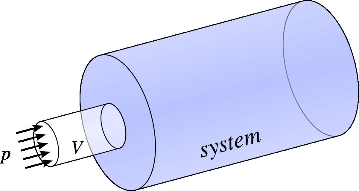
3.3.1 Entering and exiting the system: flow work ¶ Let’s imagine an open system in steady flow, containing a small water pump. In order to insert water into the pump at a given pressure, energy must be supplied to the system. Conversely, to push the water outside (at a higher pressure), the system must supply energy. How can we quantify this energy?
Consider the case of a fluid element (namely, a small quantity of fluid in transit, with volume V e l e m e n t ) V_{\mathrm{element}}) V element ) p 1 p_{1} p 1
The work W i n s e r t i o n W_{\mathrm{insertion}} W insertion
W i n s e r t i o n = p 1 V e l e m e n t W_{\mathrm{insertion}}= p_{1}V_{\mathrm{element}} W insertion = p 1 V element where W i n s e r t i o n W_{\mathrm{insertion}} W insertion ( J ) (J) ( J ) V e l e m e n t V_{\mathrm{element}} V element ( m 3 ) (m^{3}) ( m 3 )
If such a volume of fluid enters the system every second, then the system receives power in the form of work, which we call insertion power ,W ˙ i n s e r t i o n \dot{W}_{\mathrm{insertion}} W ˙ insertion
Figure 3.2: A fluid element of volume V e l e m e n t V_{\mathrm{element}} V element p p p
Diagram CC-0 Olivier Cleynen
We sometimes express it in specific form (§1.1.5):
W i n s e r t i o n = p 1 V ˙ 1 = m ˙ 1 p 1 v 1 = m ˙ p 1 v 1 W_{\mathrm{insertion}}= p_{1}\dot{V}_{1}=\dot{m}_{1}p_{1}v_{1}=\dot{m} p_{1}v_{1} W insertion = p 1 V ˙ 1 = m ˙ 1 p 1 v 1 = m ˙ p 1 v 1 w i n s e r t i o n = p 1 v 1 w_{\mathrm{insertion}}= p_{1}v_{1} w insertion = p 1 v 1 where W ˙ i n s e r t i o n \dot{W}_{\mathrm{insertion}} W ˙ insertion ( W ) (W) ( W ) w i n s e r t i o n w_{\mathrm{insertion}} w insertion ( J k g − 1 ) (J kg^{-1}) ( J k g − 1 ) m ˙ 1 \dot{m}_{1} m ˙ 1 ( k g s − 1 ) (kg s^{-1}) ( k g s − 1 ) m ˙ \dot{m} m ˙ k g s − 1 ) kg s^{-1}) k g s − 1 ) V 1 V_{1} V 1 ( m 3 s − 1 ) (m^{3}s^{-1}) ( m 3 s − 1 ) v 1 v_{1} v 1 ( m 3 k g − 1 ) (m^{3}kg^{-1}) ( m 3 k g − 1 )
Similarly, for the fluid to exit the system at the other end, the system must continuously supply a power called extraction power :
W e x t r a c t i o n = − p 2 V ˙ 2 = m ˙ 2 p 2 v 2 = − m ˙ p 2 v 2 W_{\mathrm{extraction}}= -p_{2}\dot{V}_{2}=\dot{m}_{2}p_{2}v_{2}= -\dot{m} p_{2}v_{2} W extraction = − p 2 V ˙ 2 = m ˙ 2 p 2 v 2 = − m ˙ p 2 v 2 w e x t r a c t i o n = − p 2 v 2 w_{\mathrm{extraction}}= -p_{2}v_{2} w extraction = − p 2 v 2 where the outgoing mass flow ratem ˙ 2 \dot{m}_{2} m ˙ 2 m ˙ \dot{m} m ˙ k g s − 1 ) kg s^{-1}) k g s − 1 )
The net sum of these two powers at the boundaries is called flow power , W f l o w ≡ W ˙ i n s e r t i o n + W ˙ e x t r a c t i o n W_{\mathrm{flow}}\equiv \dot{W}_{\mathrm{insertion}}+\dot{W}_{\mathrm{extraction}} W flow ≡ W ˙ insertion + W ˙ extraction
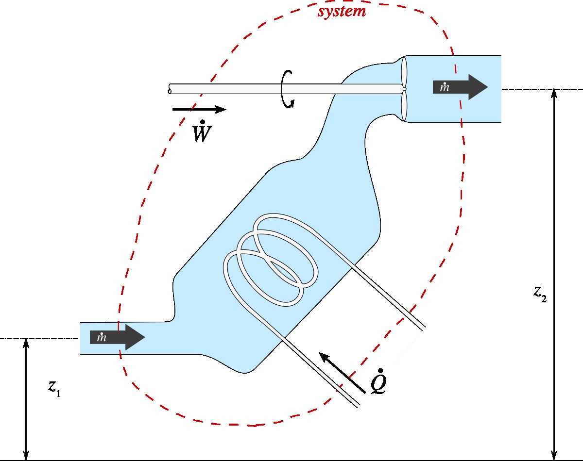
3.3.2 Energy balance ¶ Let us try to design an open system in steady flow in the most general way possible, as represented in figure 3.3. We will now account for all energy transfers within it.
When entering the system, the fluid already has an internal energy u 1 u_{1} u 1 U ˙ 1 \dot{U}_{1} U ˙ 1
U ˙ 1 = m ˙ u 1 \dot{U}_{1}=\dot{m} u_{1} U ˙ 1 = m ˙ u 1 Similarly, the fluid has a specific mechanical energy e m e c h 1 e_{\mathrm{mech}1} e mech 1 E ˙ m e c h 1 \dot{E}_{\mathrm{mech}1} E ˙ mech 1
E ˙ m e c h 1 = m ˙ e m e c h 1 = m ˙ ( 1 2 C 1 2 + g z 1 ) \dot{E}_{\mathrm{mech}1}=\dot{m} e_{\mathrm{mech}1}=\dot{m} \bigl(\tfrac{1}{2} C_{1}^{2}+ g z_{1}\bigr) E ˙ mech 1 = m ˙ e mech 1 = m ˙ ( 2 1 C 1 2 + g z 1 ) These expressions 3/6 and 3/7 have the opposite sign at the system’s outlet, where we assign them the index 2.
At this point, we have covered all of the energy forms that can be observed crossing the boundaries of an open system together with the fluid: flow work, internal energy, and mechanical energy. Since the first law states that energy is indestructible (§1.1.2), the addition of power Q ˙ \dot{Q} Q ˙ W ˙ \dot{W} W ˙
Q ˙ 1 → 2 + W ˙ 1 → 2 + ( W ˙ i n s e r t i o n + U ˙ 1 + E ˙ m e c h 1 ) + ( W ˙ e x t r a c t i o n + U ˙ 2 + E ˙ m e c h 2 ) = 0 \dot{Q}_{1\rightarrow 2}+\dot{W}_{1\rightarrow 2}+ (\dot{W}_{\mathrm{insertion}}+\dot{U}_{1}+\dot{E}_{\mathrm{mech}1}) + (\dot{W}_{\mathrm{extraction}}+\dot{U}_{2}+\dot{E}_{\mathrm{mech}2}) = 0 Q ˙ 1 → 2 + W ˙ 1 → 2 + ( W ˙ insertion + U ˙ 1 + E ˙ mech 1 ) + ( W ˙ extraction + U ˙ 2 + E ˙ mech 2 ) = 0 where all terms are expressed in watts.
Figure 3.3: An arbitrary open system. The system (whose boundaries are dashed lines, in red) is crossed from left to right by the fluid flowing with a constant mass flow rate m ˙ \dot{m} m ˙ W ˙ 1 → 2 \dot{W}_{1\rightarrow 2} W ˙ 1 → 2 Q ˙ 1 → 2 \dot{Q}_{1\rightarrow 2} Q ˙ 1 → 2
Diagram CC-0 Olivier Cleynen
We can re-express equation 3/8 in terms of directly measurable quantities:
Q ˙ 1 → 2 + W ˙ 1 → 2 + m ˙ ( p 1 v 1 + u 1 + 1 2 C 1 2 + g z 1 ) = m ˙ ( p 2 v 2 + u 2 + 1 2 C 2 2 + g z 2 ) \dot{Q}_{1\rightarrow 2}+\dot{W}_{1\rightarrow 2}+\dot{m} \bigl(p_{1}v_{1}+ u_{1}+ \tfrac{1}{2} C_{1}^{2}+ g z_{1}\bigr) =\dot{m} \bigl(p_{2}v_{2}+ u_{2}+ \tfrac{1}{2} C_{2}^{2}+ g z_{2}\bigr) Q ˙ 1 → 2 + W ˙ 1 → 2 + m ˙ ( p 1 v 1 + u 1 + 2 1 C 1 2 + g z 1 ) = m ˙ ( p 2 v 2 + u 2 + 2 1 C 2 2 + g z 2 ) or:
Q ˙ 1 → 2 + W ˙ 1 → 2 = m ˙ [ Δ u + Δ ( p v ) + 1 2 Δ ( C 2 ) + g Δ z ] \dot{Q}_{1\rightarrow 2}+\dot{W}_{1\rightarrow 2}=\dot{m}\bigl[\Delta u + \Delta (pv) + \tfrac{1}{2}\Delta (C^{2}) + g \Delta z\bigr] Q ˙ 1 → 2 + W ˙ 1 → 2 = m ˙ [ Δ u + Δ ( p v ) + 2 1 Δ ( C 2 ) + g Δ z ] q 1 → 2 + w 1 → 2 = Δ u + Δ ( p v ) + Δ e m e c h . q_{1\rightarrow 2}+ w_{1\rightarrow 2}= \Delta u + \Delta (pv) + \Delta e_{\mathrm{mech}.} q 1 → 2 + w 1 → 2 = Δ u + Δ ( p v ) + Δ e mech . where the symbols Δ \Delta Δ
Equations 3/9 and 3/11 are extremely useful in thermodynamics, because they allow us to quantify by deduction the powers involved in flows. They allow us, in particular, to predict the properties of the fluid at the outlet of a device for which we know the mechanical power and heat emissions. For example, we can determine the remaining energy in the air at the outlet of a turbine for which we know the power.
The compressor of a turbofan admits 1.5 k g s − 1 1.5 kg s^{-1} 1.5 k g s − 1 192.5 k J k g − 1 192.5 kJ kg^{-1} 192.5 k J k g − 1 0.96 m 3 k g − 1 0.96 m^{3}kg^{-1} 0.96 m 3 k g − 1 643.1 k J k g − 1 643.1 kJ kg^{-1} 643.1 k J k g − 1 8.57 × 1 0 − 2 m 3 k g − 1 8.57 \times 10^{-2}m^{3}kg^{-1} 8.57 × 1 0 − 2 m 3 k g − 1
What is the power of the compressor if its heat transfers are negligible?
We apply equation 3/10 to obtain: W 1 → 2 = − Q ˙ 1 → 2 + m ˙ [ Δ u + Δ ( p v ) + 1 2 Δ ( C 2 ) + g Δ z ] = 0 + m ˙ [ Δ u + Δ ( p v ) + 0 + 0 ] = 1.5 [ ( 643.1 × 1 0 3 − 192.5 × 1 0 3 ) + ( 30 × 1 0 5 × 8.57 × 1 0 − 2 − 0.8 × 1 0 5 × 0.96 ) ] W_{1\rightarrow 2}= -\dot{Q}_{1\rightarrow 2}+\dot{m}[\Delta u + \Delta (pv) + \frac{1}{2}\Delta (C^{2}) + g \Delta z] = 0 +\dot{m}[\Delta u + \Delta (pv) + 0 + 0] = 1.5 [(643.1 \times 10^{3}- 192.5 \times 10^{3}) + (30 \times 10^{5}\times 8.57 \times 10^{-2}- 0.8 \times 10^{5}\times 0.96)] W 1 → 2 = − Q ˙ 1 → 2 + m ˙ [ Δ u + Δ ( p v ) + 2 1 Δ ( C 2 ) + g Δ z ] = 0 + m ˙ [ Δ u + Δ ( p v ) + 0 + 0 ] = 1.5 [( 643.1 × 1 0 3 − 192.5 × 1 0 3 ) + ( 30 × 1 0 5 × 8.57 × 1 0 − 2 − 0.8 × 1 0 5 × 0.96 )]
= + 9.464 × 1 0 5 W = + 946.4 k W = +9.464 \times 10^{5}W = +946.4 kW = + 9.464 × 1 0 5 W = + 946.4 kW
The only difficulty in applying this equation concerns the proper conversion of units. Pressure and energy should always be converted from their usual units to si units.
The power is positive, as expected since the air receives the work.
In a turbine, the work would be negative.
3.3.3 Enthalpy ¶ In many cases, the terms u u u p v pv p v
We call the sum of the terms u u u p v pv p v specific enthalpy , and assign it the symbol h h h
h ≡ u + p v h \equiv u + p v h ≡ u + p v where the terms are expressed in J k g − 1 J kg^{-1} J k g − 1
Of course, the enthalpy H H H
where H H H
In practice, the term enthalpy is often used even if it refers to specific enthalpy; the symbol and context help determine which variable is being referred to.
« The decrease of the heat contents is equal to the heat value of the gained “useful work” plus the heat carried away to the outside plus the increase of kinetic energy per pound (or kilogram) of steam. »
Aurel Stodola, 1904
(where the “heat contents” are not yet named enthalpy )
Die Dampfturbinen [26 27
By using the concept of enthalpy, equations 3/9 and 3/11 are simplified to become:
Q 1 → 2 + W ˙ 1 → 2 = m ˙ ( Δ h + Δ e m e c h . ) Q_{1\rightarrow 2}+\dot{W}_{1\rightarrow 2}=\dot{m}(\Delta h + \Delta e_{\mathrm{mech}.}) Q 1 → 2 + W ˙ 1 → 2 = m ˙ ( Δ h + Δ e mech . ) q 1 → 2 + w 1 → 2 = Δ h + Δ e m e c h . q_{1\rightarrow 2}+ w_{1\rightarrow 2}= \Delta h + \Delta e_{\mathrm{mech}.} q 1 → 2 + w 1 → 2 = Δ h + Δ e mech . Thus, in an open system, we see that heat and work transfers change the enthalpy of the fluid, and not only its internal energy as in a closed system.
In a nozzle, air expands without any work or heat transfer. It enters with a specific enthalpy of 776 k J k g − 1 776 kJ kg^{-1} 776 k J k g − 1 30 k m / h ( 18.6 m p h ) 30 km/h (18.6 mph) 30 km / h ( 18.6 m p h ) 754 k J k g − 1 754 kJ kg^{-1} 754 k J k g − 1
What is the air ejection velocity?
We start from equation 3/15:
q 1 → 2 + w 1 → 2 = Δ h + Δ e m e c h . q_{1\rightarrow 2}+ w_{1\rightarrow 2}= \Delta h + \Delta e_{\mathrm{mech}.} q 1 → 2 + w 1 → 2 = Δ h + Δ e mech . Δ e m e c h . = − Δ h + 0 + 0 \Delta e_{\mathrm{mech}.}= -\Delta h + 0 + 0 Δ e mech . = − Δ h + 0 + 0 1 2 ( C 2 2 − C 1 2 ) = − Δ h \frac{1}{2} (C_{2}^{2}- C_{1}^{2}) = -\Delta h 2 1 ( C 2 2 − C 1 2 ) = − Δ h C 2 = [ − 2 Δ h + C 1 2 ] 1 2 C_{2}= [-2 \Delta h + C_{1}^{2}]^{\frac{1}{2}} C 2 = [ − 2Δ h + C 1 2 ] 2 1 So C 2 = [ − 2 × ( 754 × 1 0 3 − 776 × 1 0 3 ) + ( 30 3.6 ) 2 ] 1 2 = 209.9 m s − 1 = 755.7 k m / h = 470 m p h C_{2}= \left[-2 \times (754 \times 10^{3}- 776 \times 10^{3}) + \left(\frac{30}{3.6}\right)^{2}\right]^{\frac{1}{2}} = 209.9 m s^{-1}= 755.7 km/h = 470 mph C 2 = [ − 2 × ( 754 × 1 0 3 − 776 × 1 0 3 ) + ( 3.6 30 ) 2 ] 2 1 = 209.9 m s − 1 = 755.7 km / h = 470 m p h
Care must be used with conversions: in the equations, velocities and energies are always in si units.
3.4 Quantifying Work with an Open System ¶ 3.4.1 Work of a fluid in a slow process ¶ We have seen that when the fluid undergoes a slow process, the work done by a closed system can be quantified by carrying out the integral − ∫ p d v -\int pdv − ∫ p d v
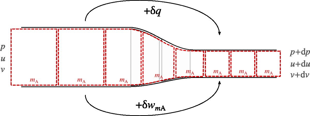
To this end, let us first observe the process undergone by a fixed mass quantity m A m_{A} m A d p dp d p d v dv d v w m A w_{m_{\mathrm{A}}} w m A
δ w m A = − p d v δ w_{m_{\mathrm{A}}}= -pdv δ w m A = − p d v during a reversible process, and where the notation δ is used to denote the infinitesimal transfer of work (work being a path quantity, see Appendix A4 p. 316).
Figure 3.4: A fixed mass quantity m A m_{A} m A p p p v v v p + d p p + dp p + d p v + d v v + dv v + d v w m A = − p d v w_{m_{\mathrm{A}}}= -pdv w m A = − p d v
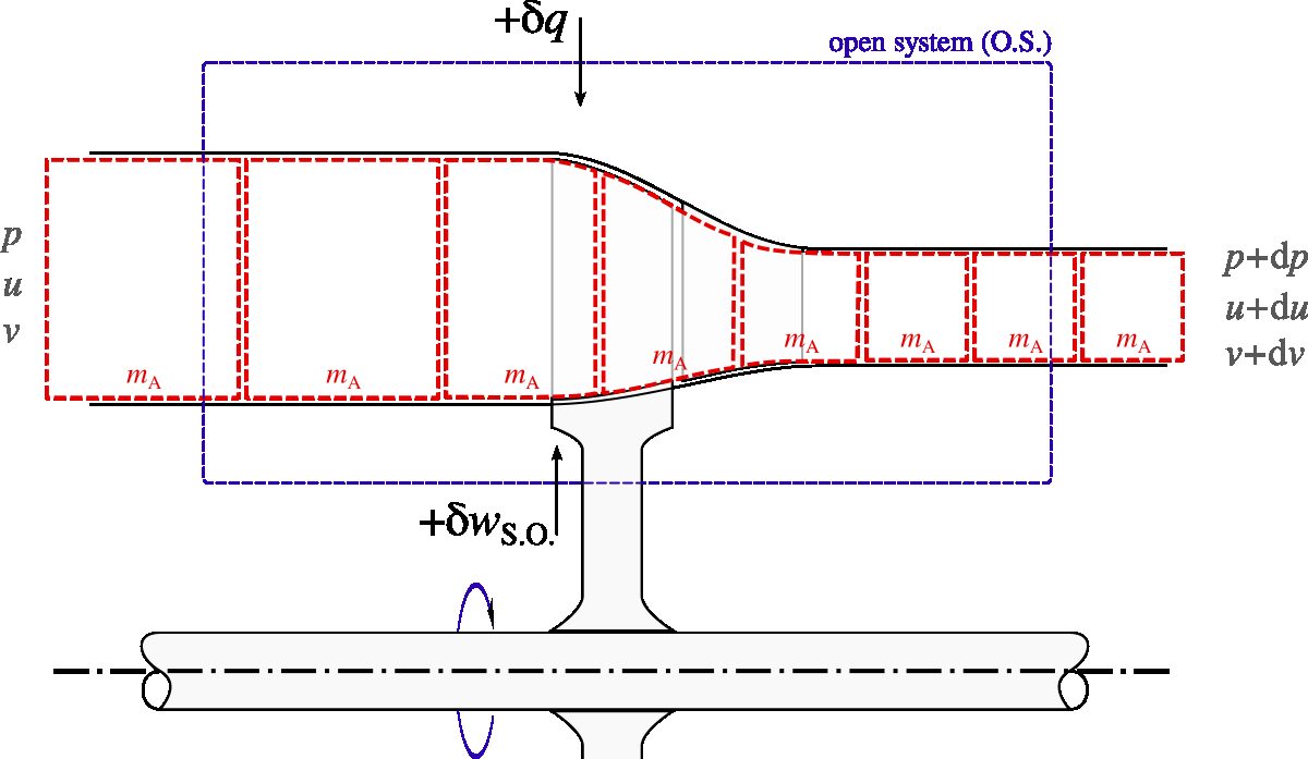
Now, let’s observe the course of this same phenomenon from the point of view of an open system (figure 3.5). What specific power δw O . S . w_{\mathrm{O.S}.} w O.S . w m A w_{m_{\mathrm{A}}} w m A
Figure 3.5: The same flow as in figure 3.4, now observed from the viewpoint of a stationary open system crossed from left to right by a steady flow. We seek to quantify the work δw O . S . w_{\mathrm{O.S}.} w O.S . m A m_{\mathrm{A}} m A w m A w_{m_{\mathrm{A}}} w m A
The open system has four work transfer forms:
The specific insertion power w i n s e r t i o n w_{\mathrm{insertion}} w insertion
w i n s e r t i o n = + p v w_{\mathrm{insertion}}= +p v w insertion = + p v The specific compression power − - − w m A w_{m_{\mathrm{A}}} w m A m A m_{A} m A
− δ w m A = − ( − p d v ) -\delta w_{m_{\mathrm{A}}}= -(-pdv) − δ w m A = − ( − p d v ) The specific extraction power w e x t r a c t i o n w_{\mathrm{extraction}} w extraction p + d p p + dp p + d p v + d v v + dv v + d v
w e x t r a c t i o n = − ( p + d p ) ( v + d v ) w_{\mathrm{extraction}}= -(p + dp)(v + dv) w extraction = − ( p + d p ) ( v + d v ) The specific power received from the outside δw O . S . w_{\mathrm{O.S}.} w O.S .
These four powers cancel each other out, since the total work transfer involved in the flow does not depend on the adopted viewpoint:
δ w O . S . + w i n s e r t i o n + ( − δ w m A ) + w e x t r a c t i o n = 0 \delta w_{\mathrm{O.S}.}+ w_{\mathrm{insertion}}+ (-\delta w_{m_{\mathrm{A}}}) + w_{\mathrm{extraction}}= 0 δ w O.S . + w insertion + ( − δ w m A ) + w extraction = 0 Therefore, we can quantify the specific power δw O . S . w_{\mathrm{O.S}.} w O.S .
δ w O . S . = − w i n s e r t i o n + δ w m A − w e x t r a c t i o n \delta w_{\mathrm{O.S}.}= -w_{\mathrm{insertion}}+ \delta w_{m_{\mathrm{A}}}- w_{\mathrm{extraction}} δ w O.S . = − w insertion + δ w m A − w extraction δ w O . S . = − p v + ( − p d v ) + ( p + d p ) ( v + d v ) = − p v − p d v + p v + p d v + d p v + d p d v = d p v + d p d v \begin{aligned}
\delta w_{\mathrm{O.S}.}&= -p v + (-pdv) + (p + dp)(v + dv) \\
&= -p v - pdv + p v + pdv + dp v + dp dv \\
&= dp v + dp dv
\end{aligned} δ w O.S . = − p v + ( − p d v ) + ( p + d p ) ( v + d v ) = − p v − p d v + p v + p d v + d p v + d p d v = d p v + d p d v And since the product d p × d v dp \times dv d p × d v
δ w O . S . = v d p \delta w_{\mathrm{O.S}.}= vdp δ w O.S . = v d p The terms d p dp d p d v dv d v
By integrating this expression 3/21 to apply it to the general case in steady flow, we obtain:
w O . S . = ∫ v d p w_{\mathrm{O.S}.}= \int vdp w O.S . = ∫ v d p W A → B = m ˙ ∫ v d p W_{\mathrm{A}\rightarrow \mathrm{B}}=\dot{m}\int vdp W A → B = m ˙ ∫ v d p in steady flow, when the process is reversible, and regardless of the heat input.
Thus, when we want to quantify reversible work in an open system, it is the integral + ∫ v d p + \int vdp + ∫ v d p − ∫ p d v -\int pdv − ∫ p d v
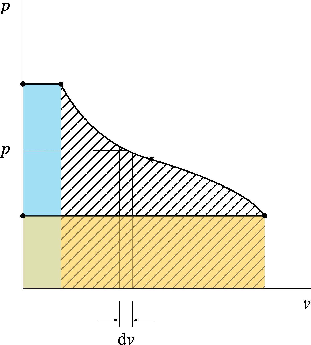
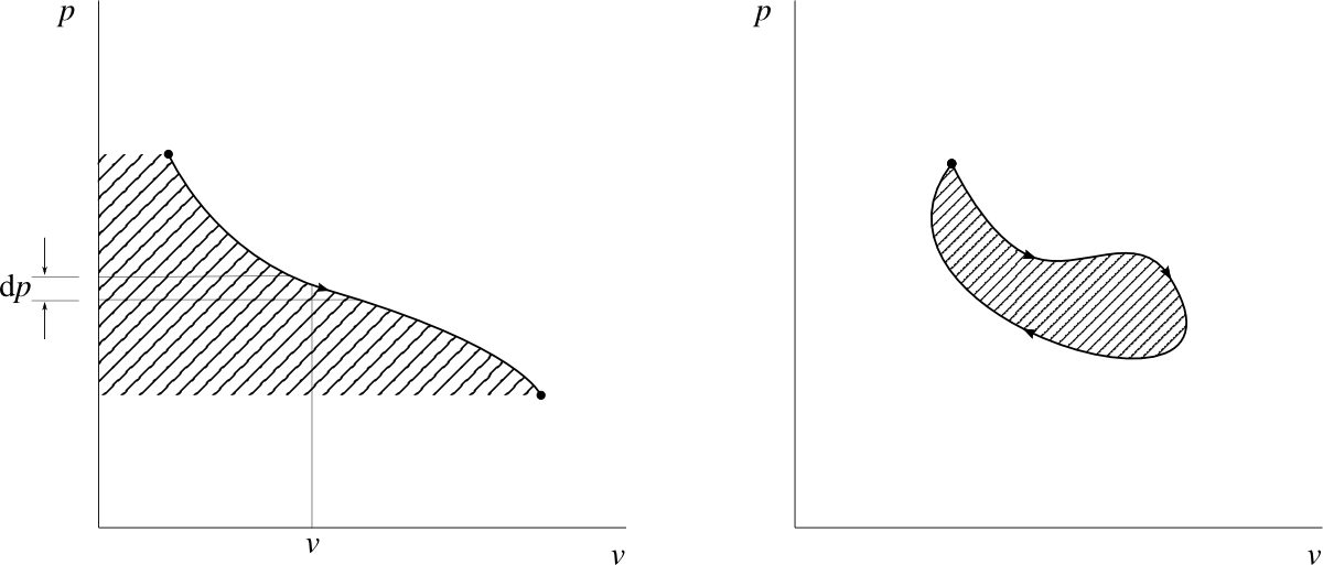
On a pressure-volume diagram, we can visualize this work by adding the insertion work and extraction work to the compression work, as shown in figure 3.6. The reversible work done in steady, reversible flow is thus visualized by the area enclosed to the left of the curve, as shown in figure 3.7.
Figure 3.6: Work received by an open system crossed by a fluid, during a slow process. The system first receives the insertion work ( p i n i . v i n i . (p_{\mathrm{ini}.}v_{\mathrm{ini}.} ( p ini . v ini . ( p f i n . v f i n . (p_{\mathrm{fin}.}v_{\mathrm{fin}.} ( p fin . v fin .
Figure 3.7: Work measured in an open system, during a reversible process. The integral of v d p vdp v d p thermodynamic cycle ), the work done is visualized by the area enclosed within the curve. In this case, the quantification is the same for closed and open systems.
Diagram CC-0 Olivier Cleynen
Diagram CC-0 Olivier Cleynen
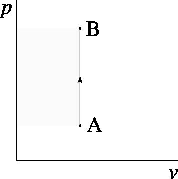
A pump slowly compresses 2 k g s − 1 ( 4.41 l b / s ) 2 kg s^{-1}(4.41 lb/s) 2 k g s − 1 ( 4.41 l b / s ) 290 p s i ) 290 psi) 290 p s i ) v L = 1 0 − 3 m 3 k g − 1 v_{L}= 10^{-3}m^{3}kg^{-1} v L = 1 0 − 3 m 3 k g − 1
The process can be drawn qualitatively (that is, without showing numerical values) on a pressure-volume diagram as follows:
We use equation 3/23, being cautious with the units. Since v v v p p p W ˙ A → B = m ˙ ∫ A B v d p = ˙ m v L ∫ A B d p = m ˙ v L [ p ] p A p B = 2 × 1 0 − 3 ( 20 × 1 0 5 − 1 × 1 0 5 ) = + 3.8 × 1 0 3 W = + 3.8 k W \dot{W}_{\mathrm{A}\rightarrow \mathrm{B}}=\dot{m}\int ^{\mathrm{B}}_{\mathrm{A}}vdp =\dot{} m v_{L}\int ^{\mathrm{B}}_{\mathrm{A}}dp =\dot{m} v_{L}[p]^{p_{\mathrm{B}}}_{p_{\mathrm{A}}}= 2 \times 10^{-3}(20 \times 10^{5}- 1 \times 10^{5}) = +3.8 \times 10^{3}W = +3.8 kW W ˙ A → B = m ˙ ∫ A B v d p = ˙ m v L ∫ A B d p = m ˙ v L [ p ] p A p B = 2 × 1 0 − 3 ( 20 × 1 0 5 − 1 × 1 0 5 ) = + 3.8 × 1 0 3 W = + 3.8 kW
This power is indeed positive, since the fluid in the system is receiving the work.
Here the specific volume v L v_{L} v L v v v
A compressor slowly compresses an air flow of 2 k g s − 1 2 kg s^{-1} 2 k g s − 1 p v 1.35 = k p v^{1.35}= k p v 1.35 = k v A = 0.8 m 3 k g − 1 v_{\mathrm{A}}= 0.8 m^{3}kg^{-1} v A = 0.8 m 3 k g − 1
The process can be drawn qualitatively on a pressure-volume diagram as follows:
Here the specific volume is a function of pressure: we have v = ( k p ) 1 1.35 = k 1 1.35 p − 1 1.35 v = \left(\frac{k}{p}\right)^{\frac{1}{1.35}}= k^{\frac{1}{1.35}} p^{-\frac{1}{1.35}} v = ( p k ) 1.35 1 = k 1.35 1 p − 1.35 1
W ˙ A → B = m ˙ ∫ A B v d p = m ˙ k 1 1.35 ∫ A B p − 1 1.35 d p = m ˙ k 1 1.35 [ 1 − 1 1.35 + 1 p − 1 1.35 + 1 ] p A p B = m ˙ ( p A v A 1.35 ) 1 1.35 1 0.25926 [ p 0.25926 ] p A p B = 2 ( 1 × 1 0 5 × 0. 8 1.35 ) 1 1.35 1 0.25926 [ ( 20 × 1 0 5 ) 0.25926 − ( 1 × 1 0 5 ) 0.25926 ] = + 7.247 × 1 0 5 W = + 724.7 k W . \dot{W}_{\mathrm{A}\rightarrow \mathrm{B}}=\dot{m}\int _{\mathrm{A}}^{\mathrm{B}}v\,\mathrm{d}p =\dot{m}\, k^{\frac{1}{1.35}} \int _{\mathrm{A}}^{\mathrm{B}}p^{-\frac{1}{1.35}}\,\mathrm{d}p =\dot{m}\, k^{\frac{1}{1.35}} \left[\frac{1}{-\frac{1}{1.35}+1}\,p^{-\frac{1}{1.35}+1}\right]_{p_{\mathrm{A}}}^{p_{\mathrm{B}}}
= \dot{m}\,(p_{\mathrm{A}} v_{\mathrm{A}}^{1.35})^{\frac{1}{1.35}}\frac{1}{0.25926}\left[p^{0.25926}\right]_{p_{\mathrm{A}}}^{p_{\mathrm{B}}}
= 2\,(1\times 10^{5}\times 0.8^{1.35})^{\frac{1}{1.35}}\frac{1}{0.25926}\left[(20\times 10^{5})^{0.25926}-(1\times 10^{5})^{0.25926}\right]
= +7.247 \times 10^{5}\,\mathrm{W} = +724.7\,\mathrm{kW}. W ˙ A → B = m ˙ ∫ A B v d p = m ˙ k 1.35 1 ∫ A B p − 1.35 1 d p = m ˙ k 1.35 1 [ − 1.35 1 + 1 1 p − 1.35 1 + 1 ] p A p B = m ˙ ( p A v A 1.35 ) 1.35 1 0.25926 1 [ p 0.25926 ] p A p B = 2 ( 1 × 1 0 5 × 0. 8 1.35 ) 1.35 1 0.25926 1 [ ( 20 × 1 0 5 ) 0.25926 − ( 1 × 1 0 5 ) 0.25926 ] = + 7.247 × 1 0 5 W = + 724.7 kW . Here the key is to correctly describe the function v ( p ) v_{(p)} v ( p )
The power of the compressor is 190 times larger than that of the pump in the previous example. Additionally, the specific volume of the air at the inlet is 800 times larger: a much larger machine will be required (it must handle a volumetric flow rate V A = m ˙ v A = 1.6 m 3 s − 1 = 1600 L s − 1 = 423 U S g a l / s V_{\mathrm{A}}=\dot{m} v_{\mathrm{A}}= 1.6 m^{3}s^{-1}= 1600 L s^{-1}= 423 US gal/s V A = m ˙ v A = 1.6 m 3 s − 1 = 1600 L s − 1 = 423 U S g a l / s
3.4.2 Work of a fluid in a fast process ¶ When the process is carried out rapidly (as is always the case in practice), we encounter the phenomena described in the previous chapter (§2.4.3): the pressure exerted on the moving walls no longer corresponds to the “average” pressure inside the fluid. The work required in compressions is greater and the work received during expansions is less than during slow processes.
Using an open system to account for energy transfers does not change the problem, of course. We do not have the means to predict analytically the work required for compression at a given speed. The problem –calculating the spatial distribution of pressure inside the fluid over time– falls within the scope of fluid mechanics, and will be solved on a case-by-case basis.
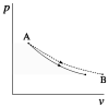
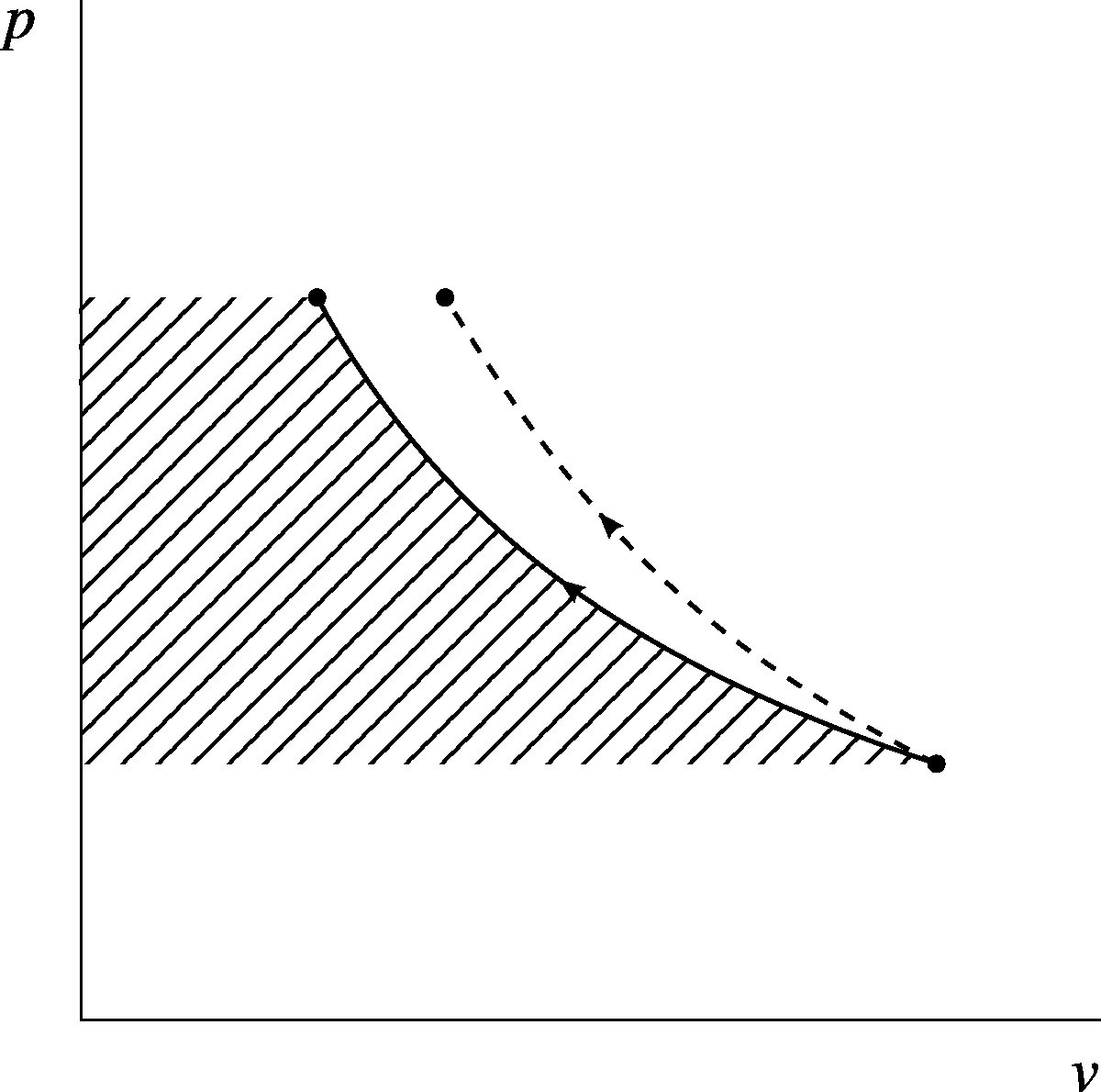
Figure 3.8: Reversible (solid line) and irreversible (dashed line) compressions represented on a pressure-volume diagram. In an open system, work transfers can be visualized with the area to the left of the curve, but only when the processes are
Diagram CC-0 Olivier Cleynen reversible.
On our pressure-volume diagrams, we represent irreversible processes with a dashed line, to clearly differentiate them from reversible processes, as shown in figure 3.8.
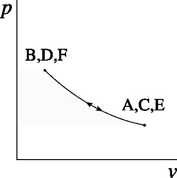
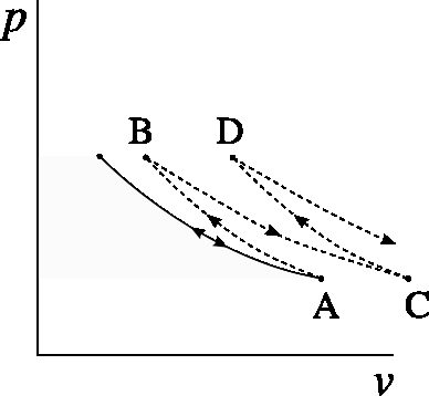
Air is continuously compressed from 1 to 20 bar in a compressor. Just after leaving the compressor, the air enters a turbine that expands it from 20 to 1 bar. After leaving the turbine, the air is again inserted into the compressor.
What will be the shape of the processes on a pressure-volume diagram?
If the processes occur infinitely slowly, the pressure and specific volume always pass through the same values during the back-and-forth movements:
Thus, the properties gradually shift on the pressure-volume diagram. Unless the processes are infinitely slow, running the compressor requires more energy than the turbine is able to provide. This excess energy is absorbed by the air, increasing its internal energy and temperature.
3.5 Quantifying Heat with an Open System ¶ With an open system, we will use the same method as with a closed system: since we cannot quantify heat transfers directly, we will always proceed by deduction. Mathematically, we simply reuse equation 3/14 to obtain:
Q 1 → 2 = m ˙ ( Δ h + Δ e m e c h . ) − W ˙ 1 → 2 Q_{1\rightarrow 2}=\dot{m}(\Delta h + \Delta e_{\mathrm{mech}.}) -\dot{W}_{1\rightarrow 2} Q 1 → 2 = m ˙ ( Δ h + Δ e mech . ) − W ˙ 1 → 2 q 1 → 2 = Δ h + Δ e m e c h . − w 1 → 2 q_{1\rightarrow 2}= \Delta h + \Delta e_{\mathrm{mech}.}- w_{1\rightarrow 2} q 1 → 2 = Δ h + Δ e mech . − w 1 → 2 for an open system.
Once again, the main challenge in quantifying a heat transfer is predicting and quantifying the change in enthalpy, Δ h \Delta h Δ h h h h the ideal gas ) and chapter 5 (liquids and vapors ).
Temperature and Amount of Heat
By Philippe Depondt
Pierre and Marie Curie University, Paris
In the second half of the 17th century, we started to concern ourselves with the matter of distinguishing between the degree of heat and the quantity of heat. This was a new question that could only arise when it became possible to reliably measure the temperature, or the “degree of heat,” of a body.
Our understanding of heat is largely tied to the sensation of hot or cold: we get burned from contact with boiling water, we feel cold when holding an ice cube in our hand. We can “feel” more or less hot, or more or less cold, an object containing “heat” would “be” more or less hot, all of this was a bit the same... In this context, the idea of a materiality of heat, the idea that a measurable quantity of heat could be transferred from one body to another and induce predictable and measurable temperature changes, remained far off!
Joseph Black (1728-1799), in Edinburgh, Scotland, then took a decisive step forward: he observed that snow does not instantly melt even though the ambient temperature can be well above the melting temperature of ice. Piles of snow, even in full sunlight, can take several days to disappear... He then posed the question: what is the temperature of the water capable of completely melting its own weight of snow at 0 ∘ C ( 3 2 ∘ F ) 0^{\circ}C (32 ^{\circ} F) 0 ∘ C ( 3 2 ∘ F ) 7 8 ∘ C ( 172. 4 ∘ F ) 78^{\circ}C (172.4 ^{\circ} F) 7 8 ∘ C ( 172. 4 ∘ F ) latent heat [39 sensible heat associated with measurable temperature changes. Beyond a clever experiment and a brilliant interpretation, a new concept had emerged.
Black continued his activities by conducting a whole series of calorimetry experiments, mixing water at different temperatures, mixing bodies of different natures at different temperatures; each time he demonstrated that the specific heat depends on the nature of the body:
We must, therefore, conclude that different bodies, although they be of the same size, or even of the same weight, when they are reduced to the same temperature or degree of heat, whatever that be, may contain very different quantities of the matter of heat; which different quantities are necessary to bring them to this level, or equilibrium, with one another.
Joseph Black, 1807 [2
He did not make any assumptions about the nature of this heat that he characterized. For most of his contemporaries, however, its apparent conservation indicated that it was a material fluid devoid of mass which Lavoisier later named caloric . In this view, this substance could be transferred from one body to another to raise the temperature of the receiving body and lower that of the giving body: some bodies (such as water) contained more of it at a given temperature than others (like oil), resulting in different specific heats. On the other hand, Black believed that the fusion of a solid or the vaporization of a liquid could be a kind of chemical combination of the caloric fluid with the matter: the caloric would then disappear as such and become “latent”.
Figure 3.9: Joseph Black conducting an experiment on latent heat during a university lecture in Edinburgh. One can imagine that he had no difficulty engaging the students, since it was about thermodynamics...
Engraving by unknown author published by Louis Figuier in 1867 (public domain)
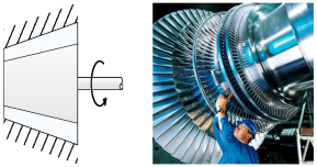
Problems ¶ Steam Turbine A steam turbine (figure 3.10) is used in a small power plant fueled by the combustion of biomass. At the inlet of the turbine, the steam has the following properties: • Pressure: 45 b a r ( 652.7 p s i ) 45 bar (652.7 psi) 45 ba r ( 652.7 p s i ) 40 0 ∘ C ( 93 2 ∘ F ) 400^{\circ}C (932 ^{\circ} F) 40 0 ∘ C ( 93 2 ∘ F ) 0.06477 m 3 k g − 1 0.064 77 m^{3}kg^{-1} 0.06477 m 3 k g − 1 2914.2 k J k g − 1 2914.2 kJ kg^{-1} 2914.2 k J k g − 1 0.75 b a r ( 10.8 p s i ) 0.75 bar (10.8 psi) 0.75 ba r ( 10.8 p s i ) 91.6 1 ∘ C ( 196. 9 ∘ F ) 91.61^{\circ}C (196.9 ^{\circ} F) 91.6 1 ∘ C ( 196. 9 ∘ F ) 2.122 m 3 k g − 1 2.122 m^{3}kg^{-1} 2.122 m 3 k g − 1 2316.3 k J k g − 1 2316.3 kJ kg^{-1} 2316.3 k J k g − 1 4 M W 4 MW 4 M W Diagram CC-0 Olivier Cleynen; Photo CC-by-sa Siemens Pressebild
w A → B = − 730.3 k J k g − 1 2 ) m ˙ = W ˙ A → B w ˙ A → B = 5.477 k g s − 1 w_{\mathrm{A}\rightarrow \mathrm{B}}= -730.3 kJ kg^{-1} 2)\dot{m} =\frac{\dot{W}_{\mathrm{A}\rightarrow \mathrm{B}}}{\dot{w}_{\mathrm{A}\rightarrow \mathrm{B}}} = 5.477kgs^{-1} w A → B = − 730.3 k J k g − 1 2 ) m ˙ = w ˙ A → B W ˙ A → B = 5.477 k g s − 1
Figure 3.10: Schematic diagram and photo of a steam turbine.
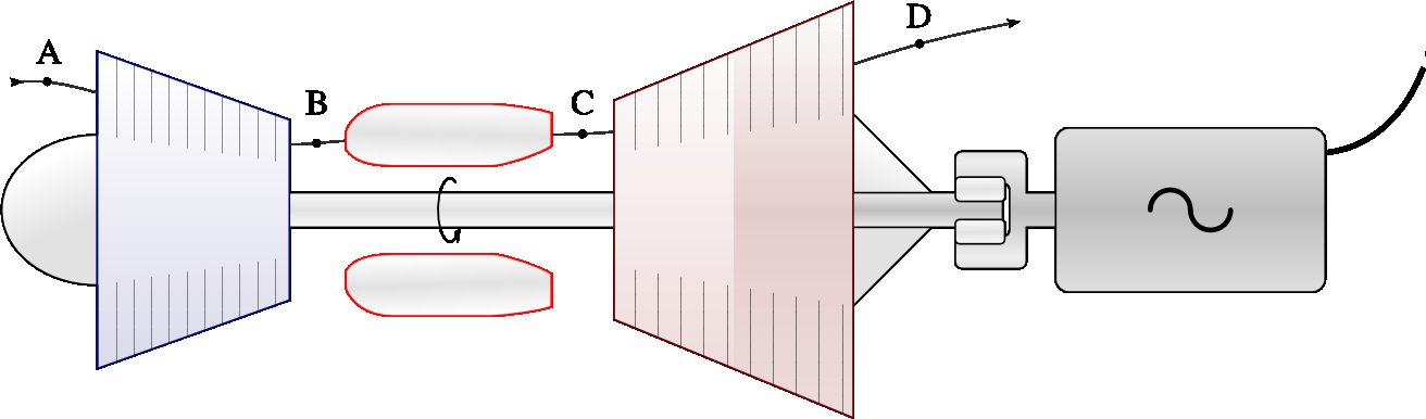
Electric Power Generator In a portable electricity-generating power plant, the electric generator is driven by a mechanical shaft. Along this shaft, there is an air compressor and a turbine (figure 3.11). This type of device, sometimes simply called a “gas turbine”, is particularly compact and efficient; however, it requires the use of refined fuels. Schematic diagram of an electricity-generating turboshaft engine Diagram CC-by-sa Olivier Cleynen The compressor brings the air from atmospheric conditions to a high pressure and temperature. Compressor inlet: • Pressure: 1 b a r ( 14.5 p s i ) 1 bar (14.5 psi) 1 ba r ( 14.5 p s i ) 0.751 m 3 k g − 1 0.751 m^{3}kg^{-1} 0.751 m 3 k g − 1 206.78 k J k g − 1 206.78 kJ kg^{-1} 206.78 k J k g − 1 35 b a r ( 507.6 p s i ) 35 bar (507.6 psi) 35 ba r ( 507.6 p s i ) 6.602 × 1 0 − 2 m 3 k g − 1 6.602 \times 10^{-2}m^{3}kg^{-1} 6.602 × 1 0 − 2 m 3 k g − 1 578.13 k J k g − 1 578.13 kJ kg^{-1} 578.13 k J k g − 1 0.1168 m 3 k g − 1 0.1168 m^{3}kg^{-1} 0.1168 m 3 k g − 1 1028.8 k J k g − 1 1028.8 kJ kg^{-1} 1028.8 k J k g − 1 1.2 b a r ( 17.4 p s i ) 1.2 bar (17.4 psi) 1.2 ba r ( 17.4 p s i ) 1.526 m 3 k g − 1 1.526 m^{3}kg^{-1} 1.526 m 3 k g − 1 460.88 k J k g − 1 460.88 kJ kg^{-1} 460.88 k J k g − 1 8 k g s − 1 8 kg s^{-1} 8 k g s − 1 2 % 2 \% 2% 85 % 85 \% 85%
1 ) W ˙ A → B = + 4.219 M W 2 ) W ˙ C → D = − 6.349 M W 3 ) E ˙ g e n e r a t o r = η g e n e r a t o r η t r a n s m i s s i o n ( W ˙ A → B + W ˙ C → D ) = − 1.774 M W 5 ) Q ˙ c o o l i n g = − W ˙ A → B − Q ˙ c o m b u s t i o n − W ˙ C → D = − 2.897 M W 1)\dot{W}_{\mathrm{A}\rightarrow \mathrm{B}}= +4.219 MW 2)\dot{W}_{\mathrm{C}\rightarrow \mathrm{D}}= -6.349 MW 3)\dot{E}_{\mathrm{generator}}= \eta _{\mathrm{generator}}\eta _{\mathrm{transmission}}(\dot{W}_{\mathrm{A}\rightarrow \mathrm{B}}+\dot{W}_{\mathrm{C}\rightarrow \mathrm{D}}) = -1.774 MW 5)\dot{Q}_{\mathrm{cooling}}= -\dot{W}_{\mathrm{A}\rightarrow \mathrm{B}}-\dot{Q}_{\mathrm{combustion}}-\dot{W}_{\mathrm{C}\rightarrow \mathrm{D}}= -2.897 MW 1 ) W ˙ A → B = + 4.219 M W 2 ) W ˙ C → D = − 6.349 M W 3 ) E ˙ generator = η generator η transmission ( W ˙ A → B + W ˙ C → D ) = − 1.774 M W 5 ) Q ˙ cooling = − W ˙ A → B − Q ˙ combustion − W ˙ C → D = − 2.897 M W
Figure 3.11: Schematic diagram of an electricity-generating turboshaft engine
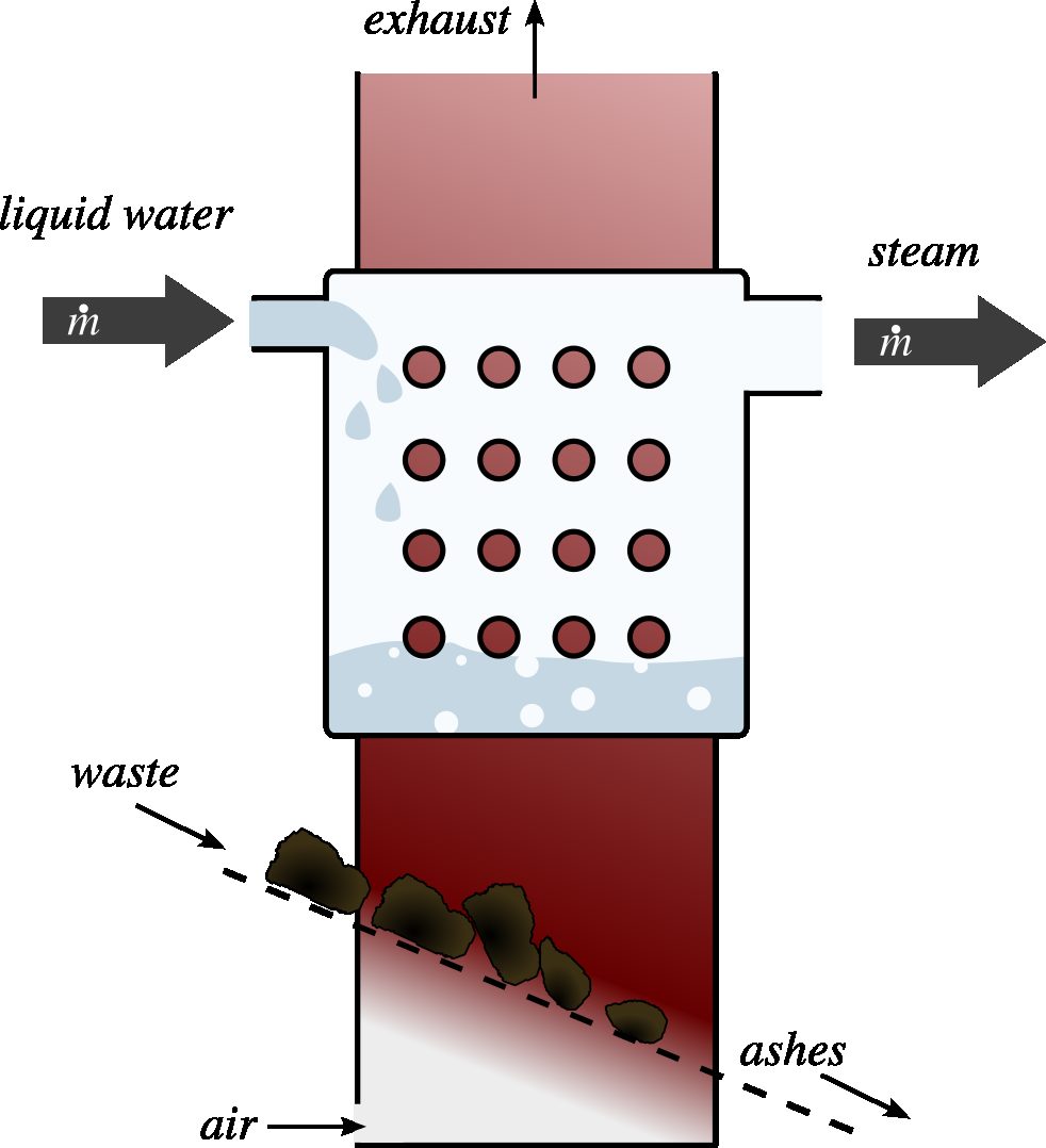
Steam Boiler A power plant provides electricity as well as industrial and domestic heat from the combustion of household waste (known as a cogeneration plant). It is equipped with a water circuit that receives some of the heat released by the combustion, at constant pressure, in a boiler. Water enters the boiler (figure 3.12) in a liquid state, pressurized at 71.89 k g f / c m 2 ( 70.5 b a r ) 71.89 kg_{f}/cm^{2}(70.5 bar) 71.89 k g f / c m 2 ( 70.5 ba r ) 1160.2 k J k g − 1 1160.2 kJ kg^{-1} 1160.2 k J k g − 1 317 t h − 1 317 t h^{-1} 317 t h − 1 3595.9 k J k g − 1 3595.9 kJ kg^{-1} 3595.9 k J k g − 1 Diagram CC-0 Olivier Cleynen The combustion of household waste generates between 9 and 11 M J k g − 1 11 MJ kg^{-1} 11 M J k g − 1 76 % 76 \% 76%
1 ) m ˙ w a s t e ≥ 92.1 t / h ≈ 203000 l b / h 1)\dot{m}_{\mathrm{waste}}\ge 92.1 t/h \approx 203 000 lb/h 1 ) m ˙ waste ≥ 92.1 t / h ≈ 203000 l b / h
Figure 3.12: Schematic diagram of a boiler operating from the combustion of waste.
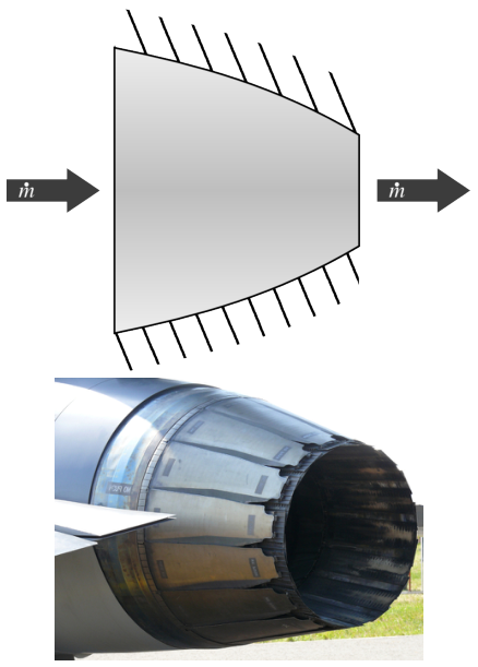
Turbine Engine Nozzle In the nozzle of a small turbojet engine, the air pressure drops while its speed increases. The nozzle (figure 3.13) is a component without any moving parts: no work is done there. Heat losses are negligible, and the air flow rate is 26 k g s − 1 ( 57.22 l b / s ) 26 kg s^{-1}(57.22 lb/s) 26 k g s − 1 ( 57.22 l b / s ) 1092 k J k g − 1 1092 kJ kg^{-1} 1092 k J k g − 1 10 m s − 1 ( 32.8 f t / s ) 10 m s^{-1}(32.8 ft/s) 10 m s − 1 ( 32.8 f t / s ) 1250.3 3 ∘ F ( 950 K ) 1250.33 ^{\circ} F (950 K) 1250.3 3 ∘ F ( 950 K ) 1.36 m 3 k g − 1 1.36 m^{3}kg^{-1} 1.36 m 3 k g − 1 2.325 k g f / c m 2 ( 2.28 b a r ) 2.325 kg_{f}/cm^{2}(2.28 bar) 2.325 k g f / c m 2 ( 2.28 ba r ) 781.85 k J k g − 1 781.85 kJ kg^{-1} 781.85 k J k g − 1 ( 1 b a r ) (1 bar) ( 1 ba r ) 944. 7 ∘ F ( 780.2 K ) 944.7 ^{\circ} F (780.2 K) 944. 7 ∘ F ( 780.2 K ) 2.55 m 3 k g − 1 2.55 m^{3}kg^{-1} 2.55 m 3 k g − 1 642.1 k J k g − 1 642.1 kJ kg^{-1} 642.1 k J k g − 1 Diagram CC-0 Olivier Cleynen; Photo CC-by-sa Ad Meskens (edited)
C 2 = 624 m s − 1 C_{2}= 624 m s^{-1} C 2 = 624 m s − 1 2250 k m / h 2250 km/h 2250 km / h 1400 m p h 1400 mph 1400 m p h 2 ) V ˙ 1 = m ˙ v 1 = 35.4 m 3 s − 1 & V ˙ 2 = 66.3 m 3 s − 1 2)\dot{V}_{1}=\dot{m} v_{1}= 35.4 m^{3}s^{-1}\&\dot{V}_{2}= 66.3 m^{3}s^{-1} 2 ) V ˙ 1 = m ˙ v 1 = 35.4 m 3 s − 1 & V ˙ 2 = 66.3 m 3 s − 1
Figure 3.13: Schematic diagram of a nozzle and installation (with variable geometry) on the Pratt & Whitney F100 engine of a Lockheed Martin F-16.
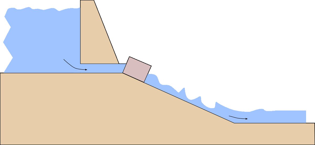
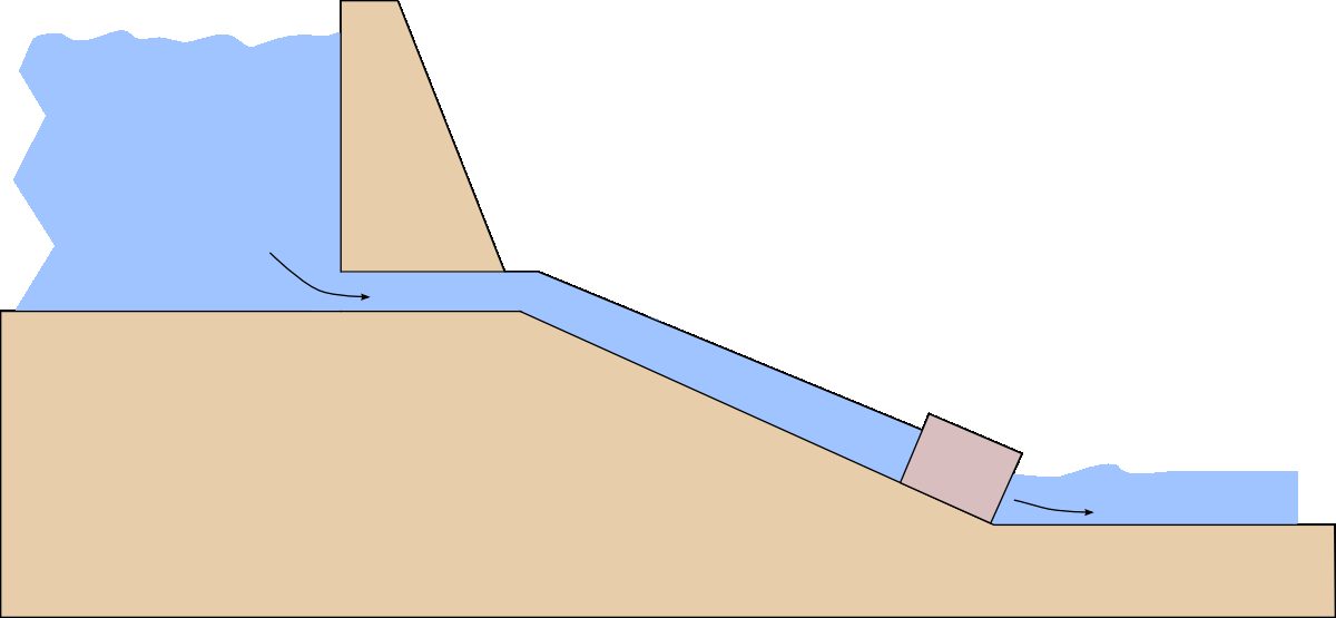
Water Turbine An engineer is working on a small hydroelectric power plant project. The objective is to harness the flow of a river ( 3170 U S g a l / s (3170 US gal/s ( 3170 U S g a l / s 12 m 3 s − 1 ) 12 m^{3}s^{-1}) 12 m 3 s − 1 ) Diagram CC-0 Olivier Cleynen In its liquid state, water is essentially incompressible (meaning its density does not change when its pressure changes). Its internal energy also varies negligibly during adiabatic compressions and expansions. The engineer first considers placing the turbine at the foot of a water reservoir, where the pressure is 4 bar and the velocity is nearly zero. The water falls through a height of 2 m ( 6.56 f t ) 2 m (6.56 ft) 2 m ( 6.56 f t ) 4 m s − 1 4 m s^{-1} 4 m s − 1 ( 1 b a r ) (1 bar) ( 1 ba r ) 25 m 25 m 25 m 82 f t 82 ft 82 f t Diagram CC-0 Olivier Cleynen 2. What would be the power transmitted in this case?
1 ) W ˙ A → B = − 3.74 M W 2 ) W ˙ A → B 2 = − 6.68 M W 1)\dot{W}_{\mathrm{A}\rightarrow \mathrm{B}}= -3.74 MW 2)\dot{W}_{\mathrm{A}\rightarrow \mathrm{B}2}= -6.68 MW 1 ) W ˙ A → B = − 3.74 M W 2 ) W ˙ A → B 2 = − 6.68 M W
Figure 3.14: Schematic diagram of a hydroelectric power plant
Figure 3.15: Schematic diagram of the modified power plant. A rigid pipe brings water to the turbine placed lower down.
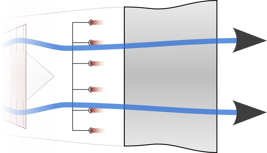
Afterburner System In order to increase the thrust it generates, the nozzle from problem 3.4 is modified to add an afterburning device (later to be studied in §10.6.2 p. 291). It consists of a set of burners that allow a second combustion of fuel to occur in the engine, just before the air enters its expansion in the nozzle (figure 3.16). After the second combustion, the air goes through its expansion and acceleration until atmospheric pressure. At the inlet, the conditions are the same as those indicated in problem 3.4. The specific power added in the form of heat by the burners reaches 1322.5 k J k g − 1 1322.5 kJ kg^{-1} 1322.5 k J k g − 1 30 M J k g − 1 30 MJ kg^{-1} 30 M J k g − 1 1406.4 k J k g − 1 1406.4 kJ kg^{-1} 1406.4 k J k g − 1 5.59 m 3 k g − 1 5.59 m^{3}kg^{-1} 5.59 m 3 k g − 1 k g / h kg/h k g / h Diagram CC-by-sa Olivier Cleynen
+ 52 % +52\% + 52% C 3 b = 950.1 m s − 1 C_{3\mathrm{b}}= 950.1\,\mathrm{m\,s^{-1}} C 3 b = 950.1 m s − 1
m ˙ f u e l = m ˙ a i r q 1 → 2 b q f u e l = 4126 k g / h = 9096 l b / h \dot{m}_{\mathrm{fuel}}= \dot{m}_{\mathrm{air}}\frac{q_{1\rightarrow 2\mathrm{b}}}{q_{\mathrm{fuel}}}= 4126\,\mathrm{kg/h} = 9096\,\mathrm{lb/h} m ˙ fuel = m ˙ air q fuel q 1 → 2 b = 4126 kg/h = 9096 lb/h
V ˙ 3 b = 145.3 m 3 s − 1 \dot{V}_{3\mathrm{b}}= 145.3\,\mathrm{m^{3}\,s^{-1}} V ˙ 3 b = 145.3 m 3 s − 1
η a f t e r b u r n i n g = 1 2 ( C 3 b 2 − C 2 2 ) q 1 → 2 b = 19.2 % \eta_{\mathrm{afterburning}}= \frac{\tfrac{1}{2}(C_{3\mathrm{b}}^{2}-C_{2}^{2})}{q_{1\rightarrow 2\mathrm{b}}} = 19.2\% η afterburning = q 1 → 2 b 2 1 ( C 3 b 2 − C 2 2 ) = 19.2%
Figure 3.16: Schematic diagram of an afterburner system. Its operation is studied in §10.6.2 p. 291.
Steam Turbine A small steam turbine produces 500 k W 500 kW 500 kW 1.35 k g s − 1 ( ∼ 3 l b / s ) 1.35 kg s^{-1} (\sim 3 lb/s) 1.35 k g s − 1 ( ∼ 3 l b / s ) 60 m s − 1 60 m s^{-1} 60 m s − 1 360 m s − 1 360 m s^{-1} 360 m s − 1 3 m 3 m 3 m 3 k W 3 kW 3 kW 3 k W 3 kW 3 kW
Δ e c = + 63 k J k g − 1 \Delta e_{c}= +63 kJ kg^{-1} Δ e c = + 63 k J k g − 1 Δ e p = + 0.0294 k J k g − 1 \Delta e_{p}= +0.0294 kJ kg^{-1} Δ e p = + 0.0294 k J k g − 1 Δ h = − 435.6 k J k g − 1 \Delta h = -435.6 kJ kg^{-1} Δ h = − 435.6 k J k g − 1
In equation 3/15, setting q 1 → 2 = 0 q_{1\rightarrow 2}= 0 q 1 → 2 = 0 w 1 → 2 w_{1\rightarrow 2} w 1 → 2 3 k W 3 kW 3 kW Δ \Delta Δ
Theoretical and Actual Turbines In the free turbine of a helicopter’s turboshaft engine, air is expanded to extract work which is transmitted to the two rotors. The characteristics are as follows: • Mass flow rate: 2 k g s − 1 2 kg s^{-1} 2 k g s − 1 0.41 m 3 k g − 1 0.41 m^{3}kg^{-1} 0.41 m 3 k g − 1 p v 1.4 = k pv^{1.4}= k p v 1.4 = k k k k 20 % 20 \% 20% 20 % 20 \% 20%
see §2.4.4 p. 49
W ˙ A → B = m ˙ k 1 1.4 [ 1 − 1 1.4 + 1 p − 1 1.4 + 1 ] p A p B = − 354.1 k W \dot{W}_{\mathrm{A}\rightarrow \mathrm{B}}=\dot{m}\,k^{\frac{1}{1.4}}\left[\frac{1}{-\frac{1}{1.4}+1} p^{-\frac{1}{1.4}+1}\right]_{p_{\mathrm{A}}}^{p_{\mathrm{B}}}= -354.1\,\mathrm{kW} W ˙ A → B = m ˙ k 1.4 1 [ − 1.4 1 + 1 1 p − 1.4 1 + 1 ] p A p B = − 354.1 kW
In the form of Δ h \Delta h Δ h
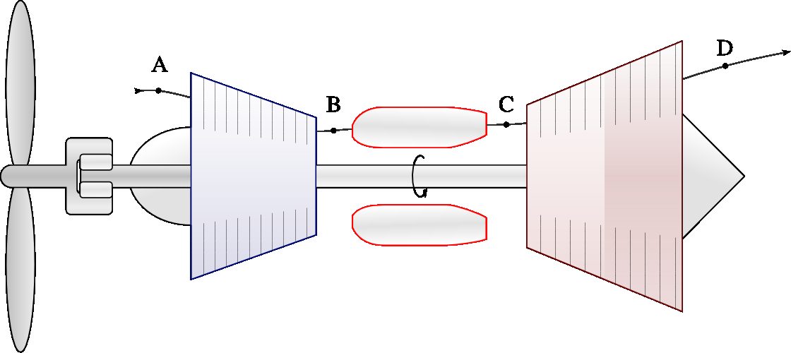
Compressor and Turbine of a Turboprop Engine The compressor within a turboprop engine (figure 3.17) admits a constant flow of air at ambient conditions ( 0.8 b a r / 11.6 p s i (0.8 bar/11.6 psi ( 0.8 ba r /11.6 p s i 1 m 3 k g − 1 ) 1 m^{3}kg^{-1}) 1 m 3 k g − 1 ) 11 b a r ( 159.5 p s i ) 11 bar (159.5 psi) 11 ba r ( 159.5 p s i ) Diagram CC-by-sa Olivier Cleynen Within the compressor, the air behaves in such a way that its properties follow the relation p v 1.4 = k p v^{1.4}= k p v 1.4 = k k k k 12 m s − 1 12 m s^{-1} 12 m s − 1 0.36 m 3 k g − 1 0.36 m^{3}kg^{-1} 0.36 m 3 k g − 1 985.8 k J k g − 1 985.8 kJ kg^{-1} 985.8 k J k g − 1 12 m s − 1 12 m s^{-1} 12 m s − 1 652.5 k J k g − 1 652.5 kJ kg^{-1} 652.5 k J k g − 1 600 k W 600 kW 600 kW
w A → B ≥ ∫ A B v d p = + 312 k J k g − 1 w_{\mathrm{A}\rightarrow \mathrm{B}}\ge \int ^{\mathrm{B}}_{\mathrm{A}}vdp = +312 kJ kg^{-1} w A → B ≥ ∫ A B v d p = + 312 k J k g − 1
& 3) see fig. 3.8 p. 71;
w C → D = − 729.3 k J k g − 1 w_{\mathrm{C}\rightarrow \mathrm{D}}= -729.3\,\mathrm{kJ\,kg^{-1}} w C → D = − 729.3 kJ k g − 1
m ˙ a i r = W ˙ p r o p e l l e r w p r o p e l l e r = W ˙ p r o p e l l e r w A → B + w C → D = 1.438 k g s − 1 \dot{m}_{\mathrm{air}}= \frac{\dot{W}_{\mathrm{propeller}}}{w_{\mathrm{propeller}}} = \frac{\dot{W}_{\mathrm{propeller}}}{w_{\mathrm{A}\rightarrow \mathrm{B}}+w_{\mathrm{C}\rightarrow \mathrm{D}}}= 1.438\,\mathrm{kg\,s^{-1}} m ˙ air = w propeller W ˙ propeller = w A → B + w C → D W ˙ propeller = 1.438 kg s − 1
Figure 3.17: Schematic diagram of a turboprop engine. These engines are studied in more detail in §10.5.4 p. 286.