2. Closed Systems - Engineering Thermodynamics

Closed Systems

A Short Treatise for Energy Accounting

Introduction¶

We wish to develop here a method of energy accounting applied to a fixed quantity of mass. This chapter 2 (closed systems) aims to answer two questions:

• How to quantify the work that can be received and provided by a body of fixed mass?

• What is reversibility, and why are we pursuing it?

2.1 Why Use a Closed System?¶

From now on, we want to describe and quantify energy transfers in fluids. We can adopt two different points of view to observe the fluid:

• Either we “cut out” a small piece of mass, which we closely follow as it moves along, and then quantify the energy transferred to it: this is what we call a closed system;

• Or we choose a fixed volume, which is constantly being crossed by a mass flow, and then quantify the energy transfers towards the volume: this is what we call an open system.

Of course, these two methods are equivalent: they will produce the same results. The choice of one or the other will simply make the analysis and quantification of transfers easier.

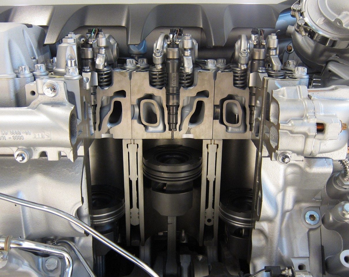
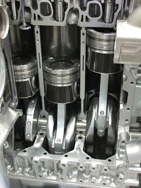
The use of a closed system is appropriate for analyzing machines with reciprocating motion (automotive engines, pumps and compressors, and generally all piston/cylinder machines). These machines divide the fluid into small quantities that are trapped in a chamber, where they are heated, cooled, compressed, or expanded (figure 2.1). It is then easy to identify a given mass quantity and quantify the transfers it undergoes.

Figure 2.1:A cutaway in a truck engine reveals three pistons in their cylinders. A closed system is a useful tool for studying the air trapped in a cylinder. The photographed engine is a diesel V8 from man.

Photo CC-by-sa Olivier Cleynen

On the contrary, to study what happens in a jet engine nozzle, for example, we would have difficulties identifying a given group of particles and quantifying the change in their properties. It would then be more convenient to use an open system, as we will study in chapter 3 (open systems).

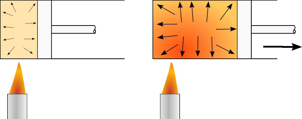
Concretely, in this chapter, we want to quantify the work that can be done by a fluid in a cylinder. A car engine provides work because the air in the cylinders provides more work by expanding on the return stroke than it received by being compressed on the intake stroke (figure 2.2). How can we generate this? In order to answer this question, we need a robust method to quantify energy transfers.

Figure 2.2:Operating principle of an engine. When heat is supplied to a fluid in a closed reservoir, it increases the forces it exerts on the walls of the reservoir. By allowing the reservoir to deform, we let the fluid perform work.

Diagram CC-0 Olivier Cleynen

2.2 Accounting Conventions¶

2.2.1 The closed system¶

We refer to a closed system as an arbitrary study subject with boundaries impermeable to mass: a given set of particles, with fixed mass. All properties of this set (pressure, temperature, volume, etc.) can change, but it always involves the same molecules, not mixed with others. For example, a gas trapped in a cylinder and compressed by a piston (figure 2.3) is perfectly described with a closed system.

Figure 2.3:A typical closed system: a fixed mass quantity in a closed reservoir. A movable wall allows to compress it; we will also allow it to receive and lose heat.

Diagram CC-0 Olivier Cleynen

2.2.2 Sign conventions¶

In order to quantify transfers, we will use the following sign convention, illustrated in figure 2.4:

• When they are positive, transfers $Q$ and $W$ indicate a receipt by the system.

• Conversely, when they are negative, transfers $Q$ and $W$ indicate a loss from the system. The system then supplies work $W$ and rejects heat $Q$ .

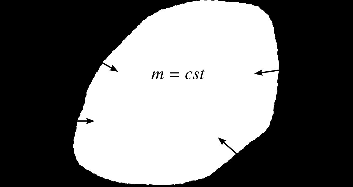
Figure 2.4:Sign conventions for a closed system. Incoming flows are positive, outgoing flows are negative; they are all represented with inward-pointing arrows. The mass quantity is constant.

Thus, in the equations, we can systematically add the terms without needing to know the direction of the changes. Transfers are accounted for like in a bank account: expenses are negative and revenues are positive.

2.3 The First Law in a Closed System¶

The first law states that energy is indestructible (§1.1.2). If we supply $100 J$ of work to a closed system and it rejects $80 J$ in the form of heat, then “its” energy has increased by $20 J$ . We call this increase the change of internal energy, $\Delta U$ . In the form of an equation, the first law in a closed system is expressed by the equation:

Q_{1\rightarrow 2}+ W_{1\rightarrow 2}= \Delta U

(2/1)

for a stationary closed system; where $\Delta U = U_{2}- U_{1}$ is the change of internal energy $(J)$ , $W_{1\rightarrow 2}$ is the work received by the system $(J)$ , and $Q_{1\rightarrow 2}$ is the heat received by the system $(J)$ .

Unfortunately, internal energy $U$ is sometimes very difficult to measure. We shall see in chapters 4 and 5 that bodies store this internal energy in different ways, and that it is intimately related to temperature. By definition, internal energy $U$ is always positive, but its variation $\Delta U$ can also be negative.

Equation 2/1 can be expressed with specific quantities:

q_{1\rightarrow 2}+ w_{1\rightarrow 2}= \Delta u

(2/2)

for a stationary closed system; where $\Delta u = u_{2}- u_{1}$ is the change of specific internal energy $(J kg^{-1})$ , $w_{1\rightarrow 2}$ is the specific work received by the system $(J kg^{-1})$ , and $q_{1\rightarrow 2}$ is the specific heat received by the system $(J kg^{-1})$ .

« Let therefore be $Q$ the whole quantity of heat which one must impart to a body while it transitions on a certain path from one state into another (whereby a withdrawn quantity of heat is counted as a negatively imparted heat quantity), so we divide this into three parts, of which the first comprehends the increase of the heat actually present in the body, the second the heat consumed for internal work and the third the heat consumed for external work. Of the first part, the same holds true as has already been said of the second, that it is independent of the manner in which the change has occurred, and therefore we can represent both parts together by a function $U$ , of which, even if we do not yet know it more closely, we know at least this much beforehand, that it is fully determined by the initial and final state of the body. »

Rudolf Clausius, 1854

Über eine veränderte Form des zweiten Hauptsatzes der mechanischen Wärmetheorie [13]

We can rewrite this equation 2/2 to express it in its differential form:

\delta q + \delta w = du

(2/3)

for a stationary closed system; where $du$ is the infinitesimal change of specific internal energy $(J kg^{-1})$ , $\delta w$ is the (specific) infinitesimal work transfer $(J kg^{-1})$ , and $\delta q$ is the (specific) infinitesimal heat transfer $(J kg^{-1})$ .

In this equation 2/3, the mathematical operators $d$ and $\delta$ have slightly different meanings: $du$ , an exact differential, represents an infinitesimal change that will integrate to $\Delta u = u_{2}-u_{1}$ ; on the other hand, an $\delta w$ , inexact differential, represents an infinitesimal transfer that will integrate to $w_{1\rightarrow 2}$ . This distinction is further elaborated in Appendix A4 p. 316.

When a fluid is brought back to its initial state (same pressure, same volume, same temperature), then it contains exactly the same amount of internal energy as before. The total energy it has received (in the form of heat or work) has therefore necessarily been returned to the surroundings in one form or another. We express this statement as follows:

Q_{\mathrm{cycle}}+ W_{\mathrm{cycle}}= 0

(2/4)

for a complete thermodynamic cycle, where $W_{\mathrm{cycle}}$ is the work received by the system $(J)$ , and $Q_{\mathrm{cycle}}$ is the heat received by the system $(J)$ .

This equation 2/4 is the reason why the first law is often stated—without adding much to our simple statement in chapter 1 — in the following way: “When a system has completed a full thermodynamic cycle, the algebraic sum of the heat it has supplied and the work it has done is zero.”

2.4 Quantifying Work with a Closed System¶

Calculating work with fluids is delicate. We will proceed in three steps of increasing complexity:

• By replacing the fluid with a spring;

• By compressing the fluid infinitely slowly;

• By compressing the fluid rapidly.

2.4.1 Work as a function of volume, with a spring¶

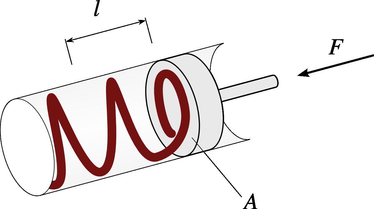
Let’s start by imagining that the fluid within a closed system behaves like a metal spring (figure 2.5). This is an interesting modeling approach to begin our study. We had seen in §1.3 that the work supplied or received by a spring is expressed as:

W_{\mathrm{A}\rightarrow \mathrm{B}}= -\int F dl

(1/11)

Today, since we are using a fluid, we want to express work in terms of pressure and volume rather than force and length.

Figure 2.5:Initially, we model the fluid inside the system with a metal spring.

Diagram CC-by-sa Olivier Cleynen

Pressure is defined as a force divided by an area:

p \equiv \frac{F}{A}

(2/5)

where $p$ is the pressure $(Pa)$ , $F$ is the force $(N)$ , and $A$ is the area of the surface on which the force acts $(m^{2})$ .

The SI unit of pressure is the Pascal,

1 Pa \equiv 1 N m^{-2}

(2/6)

but three other units are commonly used instead:

the bar:

1 bar \equiv 1 \times 10^{5}Pa

(2/7)

the kilogram-force per square centimeter, which is almost equal to the bar:

1 kg_{f}/cm^{2}= 9.806 65 \times 10^{4}Pa

(2/8)

and the pound per square inch:

1 psi = 6.894 757 \times 10^{3}Pa

(2/9)

Note that atmospheric pressure at low altitude is of the order of one bar or one kilogram-force per square centimeter $(p_{\mathrm{atm.std}.}\equiv 1 atm \equiv 1.013 25 bar \approx 14.7 psi)$ . Care is needed when reading pressure on measurement devices, which often indicate gauge pressure and not real pressure. This difference is described in Appendix A2 p. 314.

Volume can also be easily expressed. If the system is deformed by a piston with area $A$ , such that its length varies by $dl$ , we have:

dV = Adl

(2/10)

where $dV$ is the infinitesimal change in volume $(m^{3})$ , $A$ is the area of the piston surface being displaced $(m^{2})$ , and $dl$ is the infinitesimal change in length of the system corresponding to the piston displacement $(m)$ .

In the SI system of units, volume is measured in $m^{3}$ , but the student is likely accustomed to using at least one of three common units:

The liter

1 L \equiv 10^{-3}m^{3}

(2/11)

The US gallon

1 US gal \equiv 3.785 411 784 \times 10^{-3}m^{3}

(2/12)

The imperial gallon

1 imp gal \equiv 4.546 09 \times 10^{-3}m^{3}

(2/13)

Let’s now express the work of a closed system in terms of volume and pressure. By inserting equations 2/5 and 2/10 into equation 1/11, we obtain:

W_{\mathrm{A}\rightarrow \mathrm{B}}= -\int_{A}^{B} F dl = -\int_{A}^{B} \frac{F}{A} Adl

(1)

W_{\mathrm{A}\rightarrow \mathrm{B}}= -\int_{A}^{B} pdV

(2/14)

for a closed system modeled by a spring, where $W_{\mathrm{A}\rightarrow \mathrm{B}}$ is the work received by the system $(J)$ , $p$ is the (uniform) internal pressure $(Pa)$ ,

and $dV$ is the change in volume $(m^{3})$ .

In order to quantify the work done on or by the system, we only need to know the relationship between $p$ and $V$ . In this case, this function $p_{(V)}$ is directly related to the characteristic $F_{(l)}$ of the spring. The spring stiffness and its geometry (regular or progressive coils) will ultimately determine the amount of work received or supplied by the system.

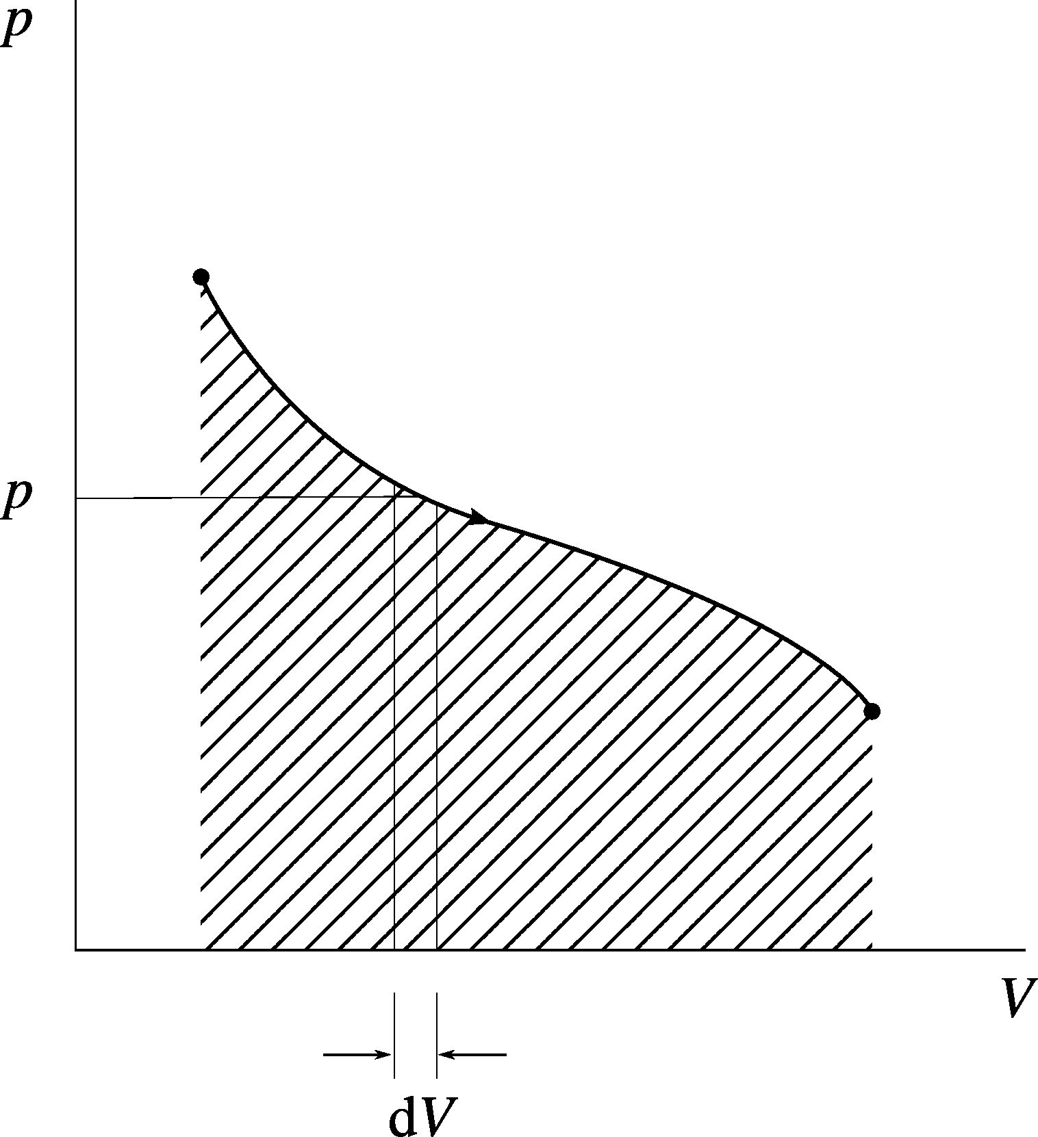
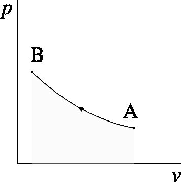
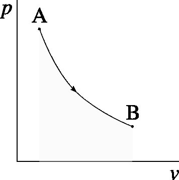
A powerful tool for understanding and analyzing work transfers is the pressure-volume diagram. In the case where the fluid is modeled by a spring, work can be visualized by the area under the curve (figure 2.6).

Figure 2.6:Pressure-volume diagram of a closed system modeled by a spring. In the case shown here, the volume is increasing (the piston moves away). The quantity $dV$ remains positive, and the work is negative: the system loses energy by doing work on the piston. This figure represents the same phenomenon as in fig. 1.3 p. 17, using different physical quantities.

Diagram CC-0 Olivier Cleynen

2.4.2 Work of a fluid in a slow process¶

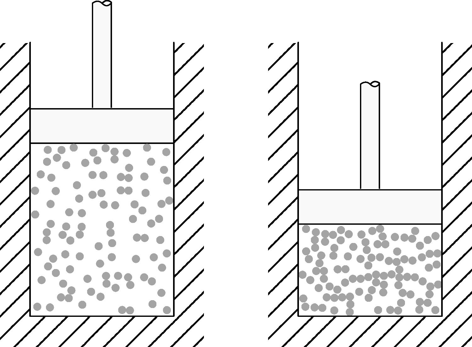
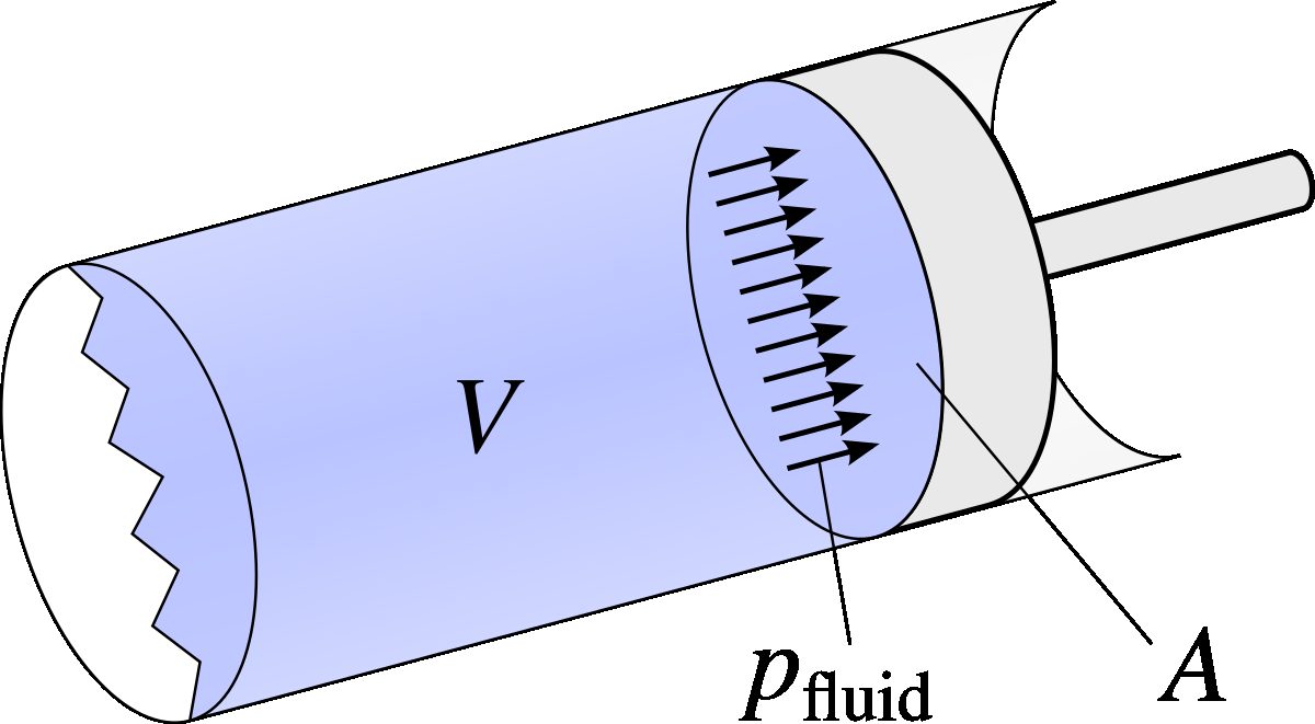
When a fluid is compressed, the molecules it is made of are brought closer to each other (figure 2.7) and the collisions between them and against the walls become more frequent. On a macroscopic scale, this increase results in an increase in pressure.

Figure 2.7:A simplistic representation of a fluid being infinitely slowly compressed without heating it. The fluid sees its temperature and pressure increase.

Diagram CC-0 Olivier Cleynen

Figure 2.8:When the piston motion is infinitely slow, the fluid behaves like a spring being compressed.

Diagram CC-by-sa Olivier Cleynen

We experimentally observe that when the motion is infinitely slow, a compressed fluid behaves exactly like a spring (figure 2.8). The condition “when the motion is infinitely slow” is of paramount importance, as we will see below.

If this condition is met, we can express the work received or supplied by the system in the same way as with the spring in the previous section:

W_{\mathrm{A}\rightarrow \mathrm{B}}= -\int pdV

(2)

A B

w_{\mathrm{A}\rightarrow \mathrm{B}}= -\int pdv

(2/15)

A for a closed system when volume changes are infinitely slow; where $w_{\mathrm{A}\rightarrow \mathrm{B}}$ is the specific work received by the system $(J kg^{-1})$ , $p$ is the (uniform) internal pressure $(Pa)$ ,

and $dv$ is the change in specific volume $(m^{3}kg^{-1})$ .

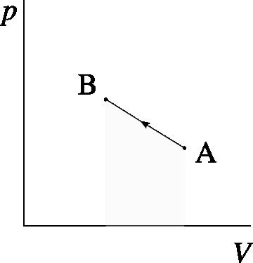
On a diagram representing pressure as a function of specific volume, this work $w_{\mathrm{A}\rightarrow \mathrm{B}}$ is represented by the area under the curve from A to B, just like in figure 2.6. The shape of the curve, that is, the relationship between $p$ and $v$ as the fluid undergoes the process, will ultimately determine the quantity $w_{\mathrm{A}\rightarrow \mathrm{B}}$ .

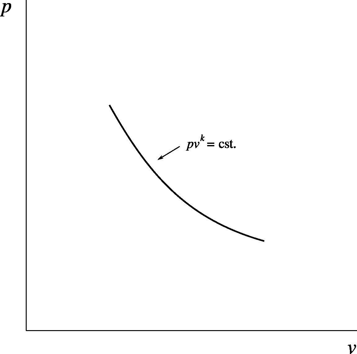
How exactly do fluids behave when they are compressed – in other words, by what type of “spring” can they be modeled? Experimentally, it is observed that when compressed, most gases have their pressure and volume related by a relation of the form $p v^{k}=$ cst. with $k$ being a constant (figure 2.9). (An exception to this trend is found with liquid/vapors when they change phase, as we will see in chapter 5.)

Figure 2.9:Properties of a gas when compressed, represented on a pressure-volume diagram. The relationship is similar to what would be obtained with a spring with progressive coils.

Diagram CC-0 Olivier Cleynen

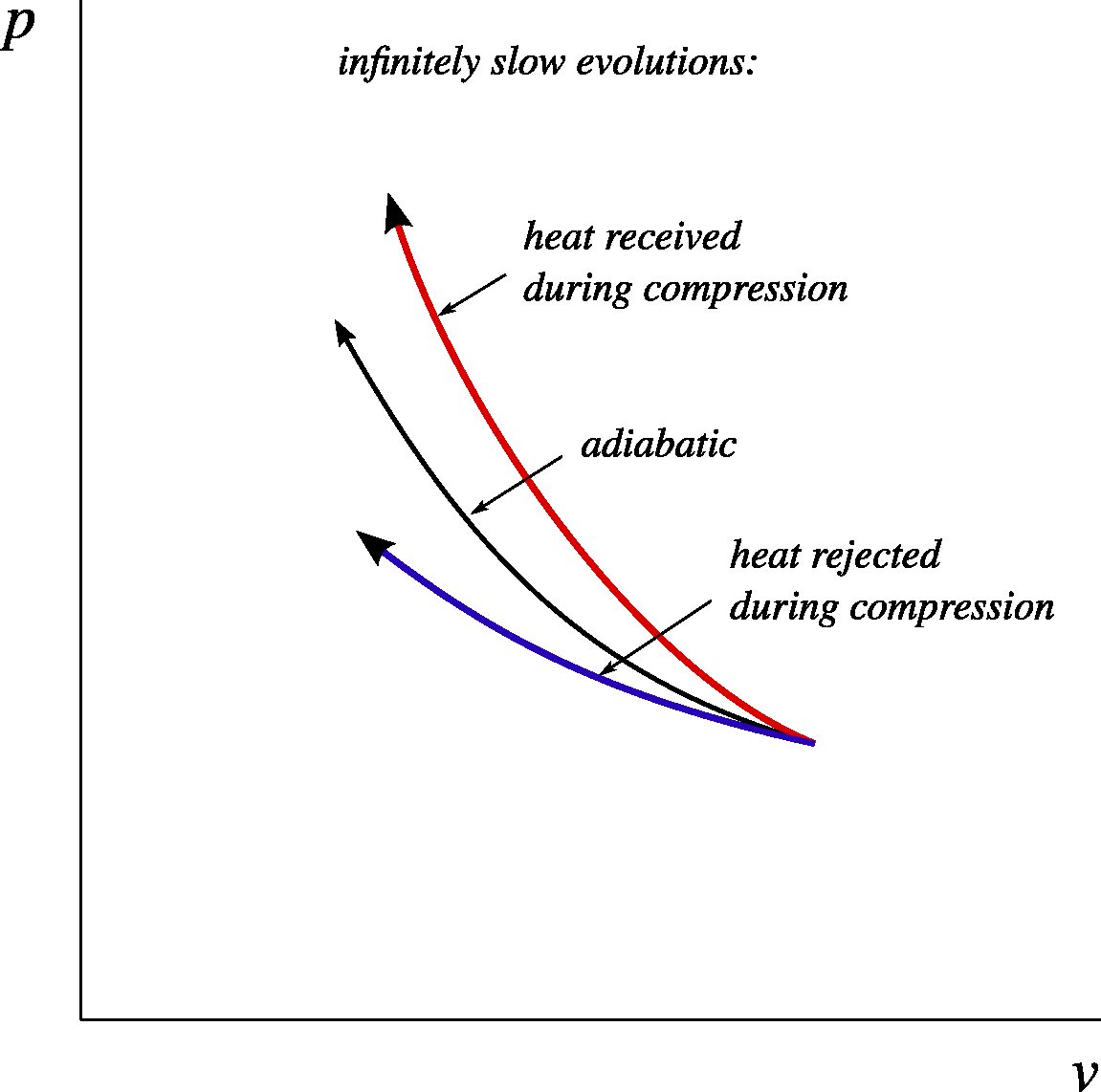
When heat is provided to the fluid while it is being compressed, its behavior becomes “stiffer”, and the pressure increases more rapidly (figure 2.10). Conversely, when heat is taken away from it during compression, the pressure increases less rapidly. These heat transfers therefore vary the amount of work required to compress the fluid between two given volumes. The case where no heat is added is called adiabatic: $Q = 0$ . Care is needed here: adiabatic does not mean “at constant temperature”. When a fluid is compressed without heat input, its temperature increases. In a diesel engine, for example, the air in the cylinders can reach $900^{\circ}C$ before combustion – which is desirable, as we will see in chapter 7 (the second law).

In the three processes of figure 2.10, the relation of the form $pv^{k}=$ cst. remains an appropriate model. The more heat is supplied during compression, the more rapidly the pressure increases – the exponent $k$ is then larger.

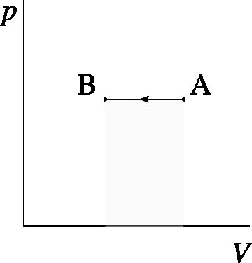
Conversely, if heat is taken away during compression, the pressure increases less rapidly and a curve closer to the horizontal (with a lower exponent $k)$ is obtained. By removing enough heat, one can even maintain a constant pressure, as we will see in chapters 4 and 5. The exponent $k$ is then zero and we have $p = p_{\mathrm{cst}.}$ .

Behavior of a fluid when infinitely slowly compressed. The more heat is supplied during compression, the more rapidly the pressure increases. The adiabatic curve represents the case where no heat transfer occurs $(Q = 0)$. — Figure 2.10:Behavior of a fluid when infinitely slowly compressed. The more heat is supplied during compression, the more rapidly the pressure increases. The adiabatic curve represents the case where no heat transfer occurs $(Q = 0)$ .

Diagram CC-0 Olivier Cleynen

Example 4

The physical quantity represented by $k$ is confusing: it is measured in $Pa m^{3.6}kg^{-1.2}$ . This is not important for us, and it is sufficient (after properly converting the input units to si!) to indicate “in si units” or $u.$ si.

Now, we can describe $p$ as a function of $v$ : $p = 10^{5}\times v^{-1.2}$ . We just have to integrate starting from equation 2/15: $w_{\mathrm{A}\rightarrow \mathrm{B}}= -\int ^{\mathrm{B}}_{\mathrm{A}}p\,\mathrm{d}v = -\int _{\mathrm{A}}^{\mathrm{B}}k v^{-1.2}\,\mathrm{d}v = -k\left[\frac{1}{-1.2+1}v^{-1.2+1}\right]_{v_{\mathrm{A}}}^{v_{\mathrm{B}}}= \frac{10^{5}}{0.2}\left[v^{-0.2}\right]_{1}^{0.167}= +2.152 \times 10^{5}\,\mathrm{J\,kg^{-1}}= +215.2\,\mathrm{kJ\,kg^{-1}}$ .

The sign of $w_{\mathrm{A}\rightarrow \mathrm{B}}$ is positive: the gas has work done to it.

The result may seem large, but it is important to remember that it is a mass-specific amount of work (§1.1.5) that needs to be multiplied by the mass of the gas to obtain a quantity in joules. At the initial conditions $(1 kg m^{-3})$ , a volume of air of $1 L$ weighs just over one gram.

Example 5

First, we need to fully know the law relating $p$ to $v$ ; then we will proceed with the integration $-\int pdv$ during the process to calculate the work. Let us start by calculating the specific volumes at the start and end: $v_{\mathrm{A}}= \frac{V_{\mathrm{A}}}{m} = \frac{0.25\times 10^{-3}}{0.3\times 10^{-3}} = 0.833 m^{3}kg^{-1}$ . Similarly, $v_{\mathrm{B}}= \frac{V_{\mathrm{B}}}{m} = 5.867 m^{3}kg^{-1}$ .

Now, we can calculate $k_{1}$ :

p_{\mathrm{A}} v_{\mathrm{A}}^{k_{1}} = p_{\mathrm{B}} v_{\mathrm{B}}^{k_{1}} \qquad \left(\frac{v_{\mathrm{A}}}{v_{\mathrm{B}}}\right)^{k_{1}} = \frac{p_{\mathrm{B}}}{p_{\mathrm{A}}} \qquad k_{1} = \frac{\ln(p_{\mathrm{B}}/p_{\mathrm{A}})}{\ln(v_{\mathrm{A}}/v_{\mathrm{B}})} = \frac{\ln(1/12)}{\ln(0.833/5.867)} = 1.2733

(3)

And with $k_{1}$ , we can calculate $k_{2}= p_{\mathrm{A}}v_{\mathrm{A}}^{k_{1}}= 12 \times 10^{5}\times 0.833^{1.2733}= 9.514 \times 10^{5}\,\mathrm{u.si}$ .

$k_{1}$ is an exponent and has no units. The units of $k_{2}$ are not interesting to us.

Although it may seem laborious, this approach of “we have a general model for the trend, what are the parameters for this specific case?” is very common in physics, and extremely useful for engineers.

We can now quantitatively describe the properties during the process: $p v^{1.2733}= 9.514 \times 10^{5}$ . We just have to carry out our usual integration:

w_{\mathrm{A}\rightarrow \mathrm{B}}= -\int _{\mathrm{A}}^{\mathrm{B}}p\,\mathrm{d}v = -k_{2}\int _{\mathrm{A}}^{\mathrm{B}}v^{-k_{1}}\,\mathrm{d}v = \frac{-9.514\times 10^{5}}{-0.2733}\left[v^{-0.2733}\right]_{0.833}^{5.867} = -1.513 \times 10^{6}\,\mathrm{J\,kg^{-1}}= -1513\,\mathrm{kJ\,kg^{-1}}.

(4)

We multiply by the mass of the gas to obtain the work: $W_{\mathrm{A}\rightarrow \mathrm{B}}= m w_{\mathrm{A}\rightarrow \mathrm{B}}= -453.8\,\mathrm{J}$ .

This calculation can be done more quickly without calculating the values of $v_{\mathrm{A}}$ , $v_{\mathrm{B}}$ , and $k_{2}$ . However, to ensure reaching the correct result, it is safer and easier to quantify $p$ and $v$ (in SI) at all stages of the process before starting an integration.

2.4.3 Work of a fluid in a fast process¶

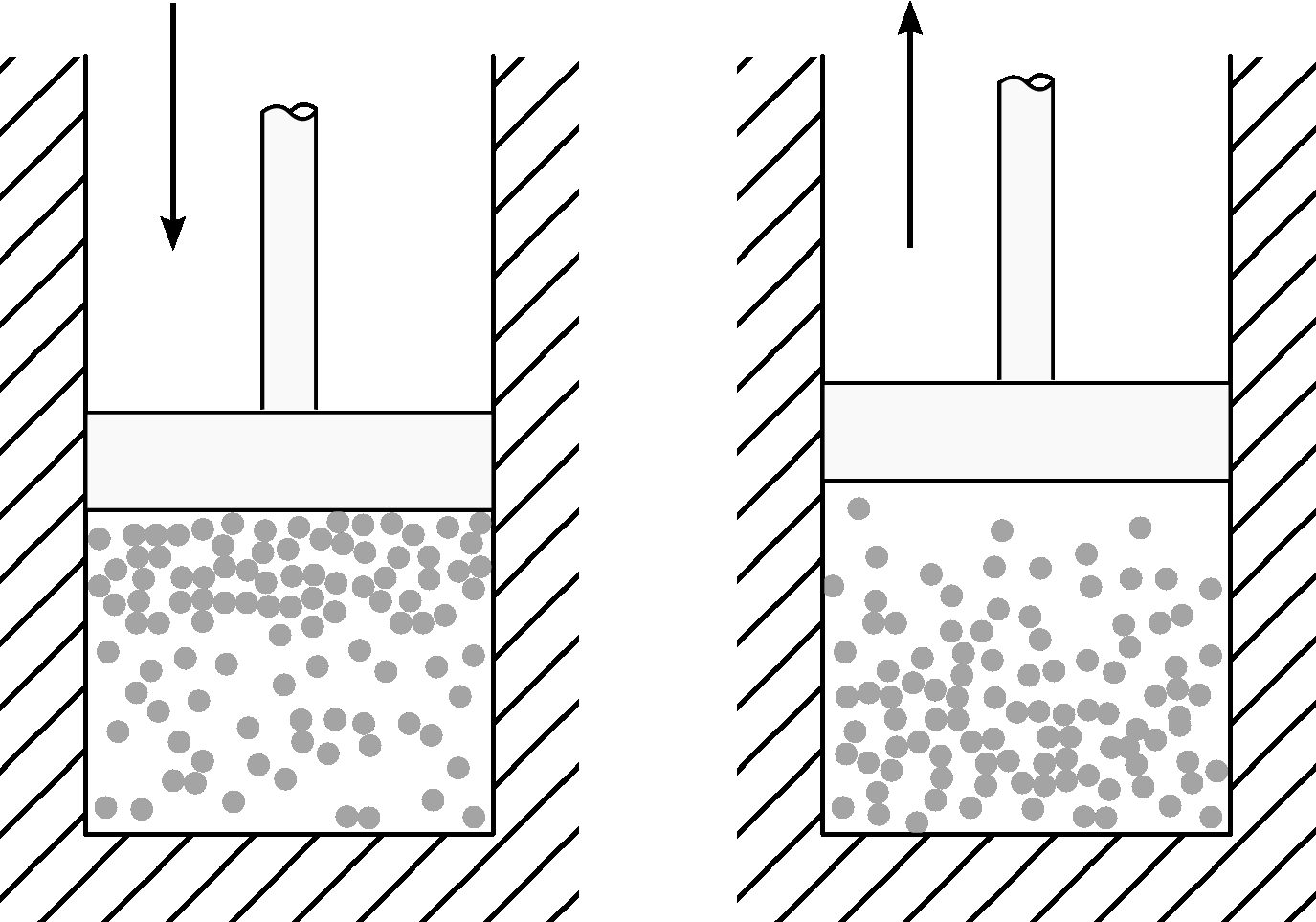
Things get more complicated when we compress and expand our fluid rapidly (figure 2.11). A complex and critically important phenomenon in thermodynamics occurs: the pressure on the wall differs from the “average pressure” inside the fluid.

Figure 2.11:Irreversible compression and expansion. When a fluid is rapidly compressed (left), the pressure on the piston wall is increased. During a rapid expansion (right), this pressure is decreased.

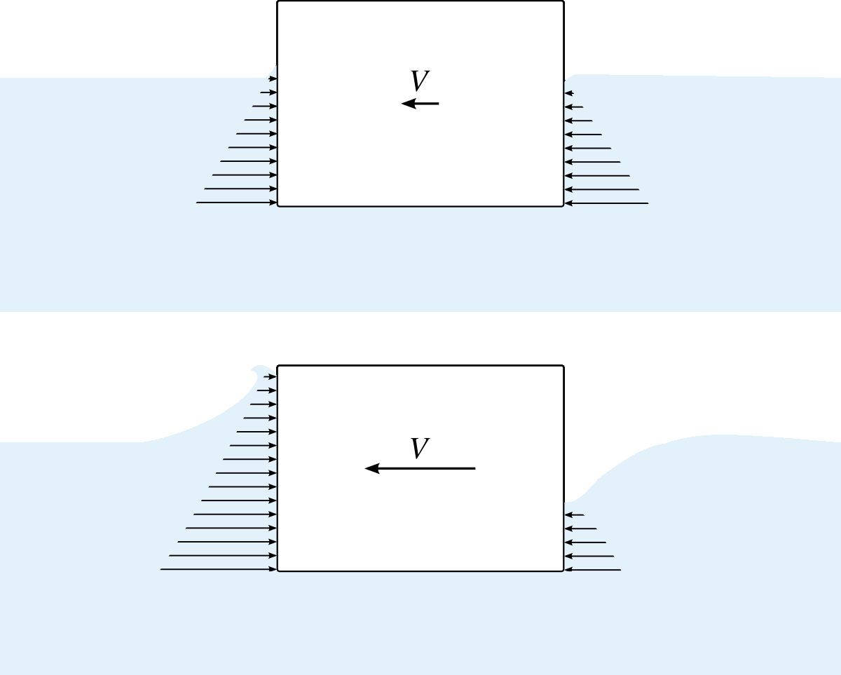
In order to describe what happens inside the fluid, we can take the example of water in a bathtub being pushed with hands – like the object shown in figure 2.12 being moved in liquid water. When the object is moved away and brought closer abruptly, the pressure on its walls is not the same as when it is moved slowly.

In each case, the amount of work done on the fluid during compression is larger, and the amount of work done by the fluid during expansion is smaller.

We call this phenomenon irreversibility. It will be a great challenge in our quantitative study of thermodynamics and will make our conversions of work and heat even more difficult.

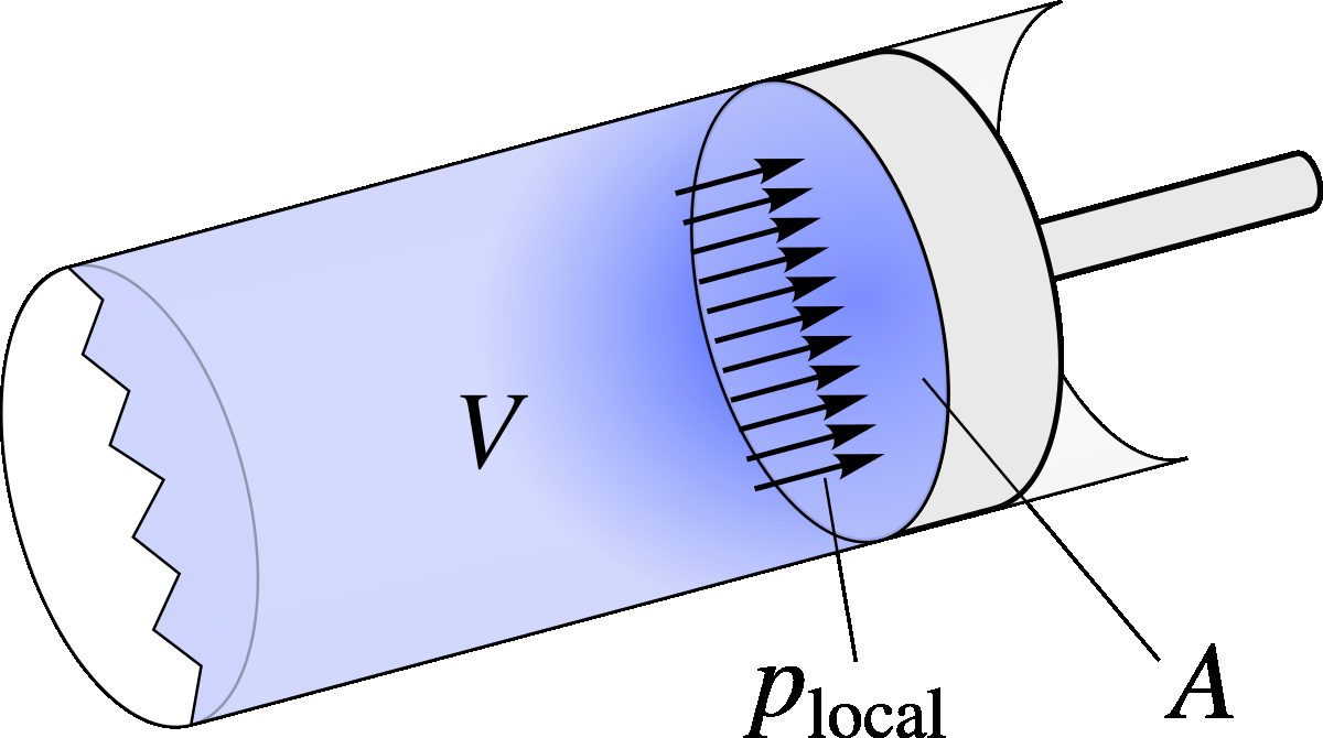
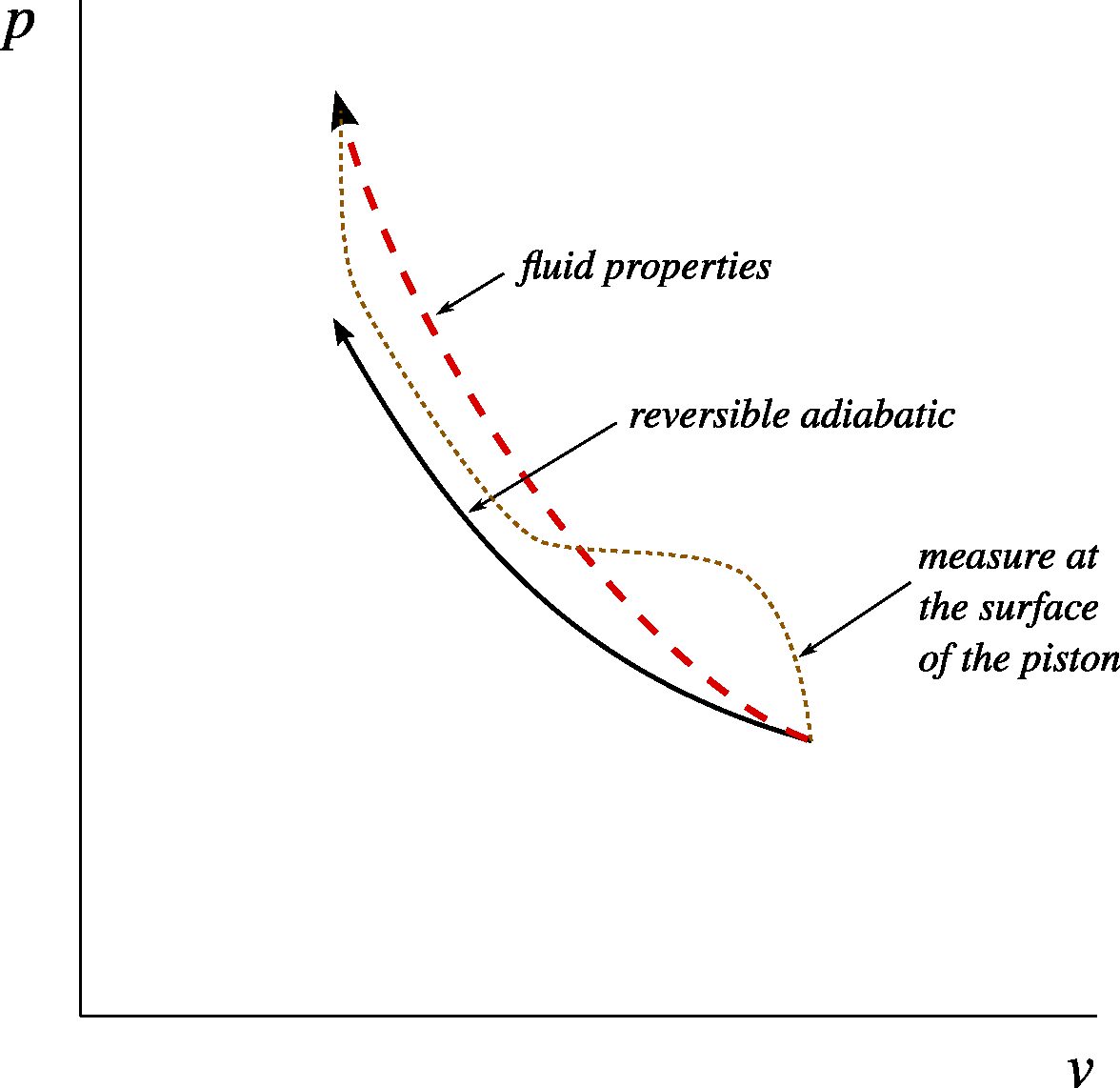
What happens in the cylinder filled with fluid when it is not compressed infinitely slowly? During a rapid compression, the pressure on the piston wall is greater than the average pressure inside the cylinder (figure 2.13). More energy is expended than necessary to carry out the displacement.

We could thus say that when compressed and expanded abruptly, a fluid behaves like a “fragile” spring, inside which something changes: it is not able to fully return all the mechanical energy it has stored.

If the received work is not equal to the work returned, then where did the excess energy go? This surplus of energy, supplied in the form of work by the piston, is converted into heat inside the fluid during the movements.

Figure 2.12:A solid object being moved in a water tank, with slow motion (above) and with fast motion (below). During fast motion, the pressure forces aiding the movement are weaker, and the forces opposing the movement are greater. In the limit of infinitely slow motion, these forces are equal.

Diagram CC-0 Olivier Cleynen

Figure 2.13:Compressed fluid abruptly. The local pressure at the piston surface is higher than it would have been with slow movement.

Diagram CC-by-sa Olivier Cleynen

The process traced on a pressure-volume diagram (figure 2.14) is much more complex than in the case of an infinitely slow process. The average pressure inside the fluid increases more rapidly than it would in a slow motion.

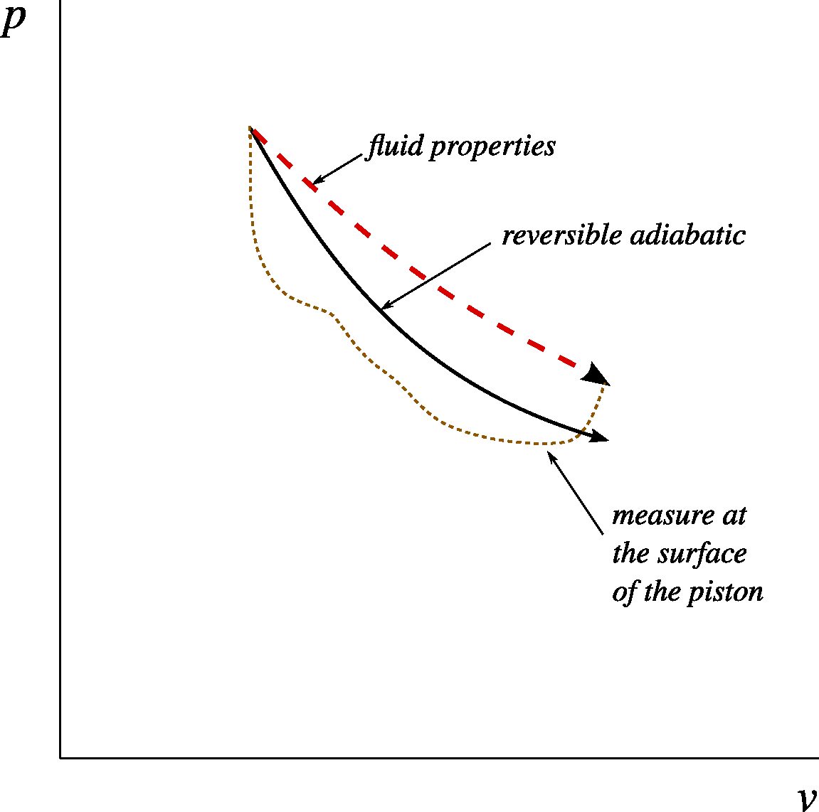
During expansion, the opposite phenomenon occurs (figure 2.15): a zone of lower pressure forms in front of the piston wall, and the work done by the fluid on the piston is less than it would have been in the reversible case.

Figure 2.14:Irreversible adiabatic compression on a pressure-volume diagram. We draw the curve with dashes: it is not a continuous series of states because the fluid pressure is not homogeneous during the process. The path the fluid would have followed if the compression had been infinitely slow is represented with a solid line. During compression, the “surplus” of work supplied by the piston is converted into heat, even though the gas is perfectly isolated.

Diagram CC-0 Olivier Cleynen

Figure 2.15:Irreversible adiabatic expansion on a pressure-volume diagram. The work received by the piston is less than it would have been with a slow motion. The path followed by the fluid is represented with dashes, because the pressure is not homogeneous during the movement.

Diagram CC-0 Olivier Cleynen

From a quantitative point of view, the more abrupt the movements on the fluid, the more the process will resemble one with heat input (“hardening” of the fluid and increase in the exponent $k$ during compressions, decrease in the exponent $k$ during expansions).

However, the work done on or by the fluid can no longer be simply calculated by integral, since the pressure inside the cylinder is not homogeneous at all. It is the pressure at the piston surface that would allow this work to be calculated. Unfortunately, no simple mathematical relationship describes this relationship between pressure and volume. An experimental measurement must be made each time.

2.4.4 Reversibility¶

Let’s take a few moments to reflect on what we have just described. Every time we compress a fluid “too quickly,” something happens that prevents us from recovering our work.

From an engineering perspective, a slow process is a limit case: one where dissipations are minimized. For example, the work required to compress a gas to 10 bar is minimal when the compression is reversible. Similarly, a turbine in which the expansion is reversible will extract the maximum work from a compressed fluid. On the contrary, in a car shock absorber, processes are made highly irreversible so that it does less work on the return path than was done on it on the outbound journey.

From a physics standpoint, the phenomenon of irreversibility is fascinating. Indeed, we start from collisions of molecules, a completely reversible phenomenon, to create an irreversible process: one that only goes in one direction! In order to bring the gas back to the state it was in before being abruptly compressed, we are forced to transfer heat away from it. It is surprising that without going against Newton’s laws, we have created a situation where we cannot go back by “doing the opposite”. Are there other irreversible processes? Can we quantify irreversibility? We will attempt to answer these questions in chapters 7 (the second law) and 8 (entropy).

In the meantime, we shall agree that three conditions must be met for a process to be reversible:

The process must occur without friction. There should be no friction in the mechanical elements (for example, between piston and cylinder).
The pressure in the fluid must be homogeneous. The movement of the walls must therefore be infinitely slow, and the fluid must move without turbulence or internal friction.
The temperature difference between the fluid and its environment must be infinitely small. If heat is supplied or rejected, it must be transferred infinitely slowly.

These three conditions obviously exclude any real process—and in particular, any practical application in an engine! However, we will use them to establish an ideal theoretical limit for all of the real processes that we will study.

2.5 Quantifying Heat with a Closed System¶

At the risk of frustrating the student, we must immediately admit that we cannot directly quantify heat transfers. We will always proceed by deduction: by quantifying the change in energy and subtracting the work transfers, we obtain the amount of heat that has been transferred. Mathematically, in a closed system, we simply reuse equation 2/1 to obtain:

Q_{1\rightarrow 2}= \Delta U - W_{1\rightarrow 2}

(2/16)

q_{1\rightarrow 2}= \Delta u - w_{1\rightarrow 2}

(2/17)

for a closed system.

The entire difficulty in quantifying a heat transfer is now to predict and quantify the change in internal energy, $\Delta U$ . For gases, $U$ is simply proportional to temperature; for liquids and vapors, the relationship is more complex. We will learn to quantify energy in fluids in chapters 4 (the ideal gas) and 5 (liquids and vapors).

A Bit of History

the Compound Engine

In the 1830s, the steam engine had just revolutionized the landscape and the economic network of Great Britain. Almost everything traveled by rail: passengers, crops, coal, industrial products. These trains were hauled by steam engines, of monumental dimensions and deplorable efficiency — ninety-seven percent of the energy released by coal was lost in the chimneys. This was not a big issue: coal and water were abundant, and it was sufficient to make punctual stops along the railway lines to replenish the machines.

Figure 2.16:SS Savannah, in the first steam-powered transatlantic crossing in 1819, which was completed under sail.

Image by Hunter Wood (public domain, 1819)

At sea, however, wind was still being used for propulsion. In order to connect two continents by engine power (meaning without tacking!), two problems had to be solved.

The first problem is that the engines consumed a lot of water. Sea water, although abundant, was unusable in its natural state because the salt and limestone deposits resulting from its boiling clogged the boilers and posed a serious risk of explosion. In order to use it in boilers, it was therefore necessary to desalinate it, a very energy-intensive operation. The problem was solved with the use of condensers, which locomotives had done away with because of space constraints. Now, when steam had done its work in the cylinders, it was no longer simply discharged into the atmosphere, but instead cooled in large condensers before being compressed and reintroduced into the boiler. The water circulated cyclically throughout the engine – one would only need to compensate for leaks.

The second problem was more serious and more difficult to solve: how to increase efficiency? It was not just a financial question: the first steam-powered transatlantic ship, the SS Savannah, was so inefficient that it completed its crossing under sail, even though it was carrying only the coal for its engine!

In order to increase the efficiency of an engine of given capacity, we seek to increase the amount of work generated by each kilogram of steam, which can be approximated by the relation 2/15:

w_{\mathrm{A}\rightarrow \mathrm{B}}= -\int_{\mathrm{A}}^{\mathrm{B}} p\, dv

(5)

The first thing to do is to increase the pressure $p_{\mathrm{A}}$ of the steam, that is, its pressure before it begins to expand in the cylinders. This is not an easy task: raising the boiler pressure increases the structural stresses it undergoes, hence its cost, and reduces its efficiency as the walls must be thickened and strengthened.

Next, one can try to increase $\Delta v$ , the total change in volume during the piston movement. In other words, it is necessary to increase the volume swept by the cylinders. Once again, this is not an easy task.

On one hand, increasing the cylinder diameter (in order to increase the area $A$ ) subjects the pistons to a greater force $F_{\mathrm{A}}$ for a given pressure $p_{\mathrm{A}}$ (2/5):

p \equiv \frac{F}{A}

(6)

By increasing the transmitted force, the structural limits of the engine mechanics are quickly reached.

On the other hand, increasing the piston travel lengthens the pistons and makes the connecting rod and crankshaft mechanisms significantly heavier. Additionally, the pressure and volume of the steam are linked: they roughly follow a relationship of the form $pv^{k_{1}}= k_{2}$ during expansion. In other words, pressure decreases when the volume is increased: as the cylinder is lengthened, the work gains become increasingly small.

The compound engine addresses this issue by using multiple cylinders in series (see figure 2.17). The high-pressure steam first drives a piston of small diameter (thus limiting the force exerted on the mechanism). It is then transferred to another cylinder of larger diameter. This cylinder allows for the same force to be obtained with a lower pressure; it sweeps a larger volume.

Figure 2.17:Cylinders in series, known as compound.

Diagram CC-by-sa Olivier Cleynen

By increasing the total volume swept by the expanding steam, more work can be extracted from the compressed steam without oversizing the crankshaft or overloading the pistons.

With such an engine, the merchant navy was able to look beyond coastal shipping: it seized upon this new technology which experienced immediate success. From two cylinders in series (double compound) it moved to three, and sometimes even four (quadruple compound!), in order to extract ever more energy from steam, in the form of work.

Enthusiastic shipowners could now boast that they now only needed to burn one sheet of paper to move one ton of cargo one mile. Even though it was understood that the said paper is very thick, progress had been made. Soon, the tea from the East Indies would arrive in the Londonian teacups – the British Empire now had the machinery required to power its formidable economic network.

Figure 2.18:Different steam compound systems.

Images by Prof. William Ripper, 1889 (public domain)

Problems¶

Exercise 2.1

Simple Processes (An exercise simply designed to practice the sign conventions and vocabulary of the chapter.) A mass of $400 g$ of water is placed in a sealed reservoir. It undergoes a process during which it receives $50 kJ kg^{-1}$ of heat, and so its internal energy increases by $4 kJ$ . 1. Did it receive or supply work, and how much? This same mass is then supplied with $800 J$ of work in an adiabatic manner. 2. What is the change in its specific internal energy?

Answer

$W_{\mathrm{A}\rightarrow \mathrm{B}}= \Delta U - mq_{\mathrm{A}\rightarrow \mathrm{B}}= -16 kJ$ (so the work is done)
$\Delta u = q_{\mathrm{B}\rightarrow \mathrm{C}}+ w_{\mathrm{B}\rightarrow \mathrm{C}}= 0 + \frac{W_{\mathrm{B}\rightarrow \mathrm{C}}}{m} = +2 kJ kg^{-1}$ .

Exercise 2.3

Truck Pneumatic Suspension The pneumatic suspension system of a truck trailer can be modeled with an air cylinder. When the trailer is loaded, the piston attached to the trailer descends inside the cylinder attached to the wheel axle, compressing the air trapped inside (figure 2.19). Initially, the truck is loaded very gradually. The air inside the cylinder neither loses nor receives heat. Its characteristics then change according to the relationship $pv^{1.4}= 5.438 \times 10^{4}$ (in si units). The compression starts at $p_{\mathrm{A}}= 2.5 bar (36.26 psi)$ . Once the loading has been completed, the pressure has risen to $p_{\mathrm{B}}= 10 bar (146 psi)$ . 1. Draw the process qualitatively (that is, without showing numerical values) on a pressure-volume diagram. 2. The work $W$ done by a force $\vec{F}$ over a displacement $l$ is expressed as $W \equiv \vec{F} ⋅\vec{l}$ suspension system. The piston, at the center, compresses a mass of air (in blue) when the trailer is loaded. Diagram CC-0 Olivier Cleynen From this equation, express the work done on a body of fixed mass in terms of its specific volume and internal pressure. 3. How much energy did the gas receive during loading? 4. How much energy would the gas give back if the truck were unloaded very gradually? The truck is unloaded abruptly and the piston rises quickly until the final pressure $p_{\mathrm{C}}$ drops back to its initial value $p_{\mathrm{C}}= p_{\mathrm{A}}= 2.5 bar$ . 4. Draw the process qualitatively on the previous pressure-volume diagram. 5. What can be done to bring the gas back to the exact state it was in before loading?

Answer

see §1.3 p. 16 & §2.4.1 p. 36
$v_{\mathrm{A}}= 0.336 m^{3}kg^{-1}$ and $v_{\mathrm{B}}= 0.125 m^{3}kg^{-1}$ ; so $w_{\mathrm{A}\rightarrow \mathrm{B}}= -k[\frac{1}{-0.4} v^{-0.4}]^{v_{\mathrm{B}}}_{v_{\mathrm{A}}}= +102.1kJkg^{-1}.$
$w_{\mathrm{B}\rightarrow \mathrm{A}}= -w_{\mathrm{A}\rightarrow \mathrm{B}}$
Cooling at constant pressure, for example.

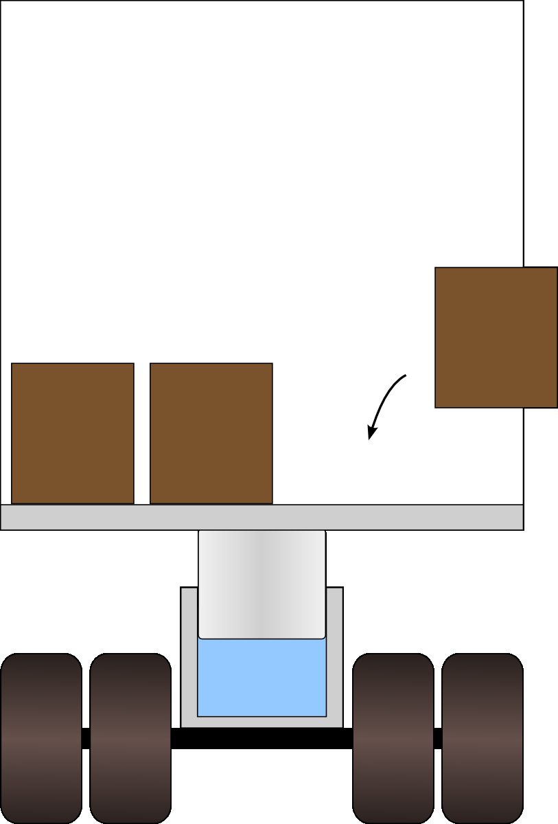
Figure 2.19:Schematic modeling of a truck pneumatic suspension system. The piston, at the center, compresses a mass of air (in blue) when the trailer is loaded.

Exercise 2.4

Air Compressor In a small air compressor (figure 2.20), a piston compresses a fixed mass of air slowly and without friction. The cylinder is equipped with fins, which are designed for heat dissipation. Thus, the compression is done at constant internal energy. We spend $150 kJ kg^{-1}$ of work in order to compress the air. 1. What is the heat transfer during compression? Before starting the compression, the air is at atmospheric pressure and density $(1 bar$ ; $1.2 kg m^{-3})$ . The diameter of the cylinder is $5 cm (1.97 in)$ and its inner depth is $15 cm (5.91 in)$ . 2. What is the mass of air included in the cylinder? During compression, it is observed that pressure and specific volume are related by the relation $pv = k$ (where $k$ is a constant). 3. To which pressure can the air be compressed at the end of the compression? Diagram CC-by-sa Christophe Dang Ngoc Chan & Olivier Cleynen

Answer

$q_{\mathrm{A}\rightarrow \mathrm{B}}= \Delta u - w_{\mathrm{A}\rightarrow \mathrm{B}}= -w_{\mathrm{A}\rightarrow \mathrm{B}}$ . $2) m = \frac{V_{\mathrm{A}}}{v_{\mathrm{A}}} = 3.534 \times 10^{-4}kg 3) \frac{v_{\mathrm{B}}}{v_{\mathrm{A}}} = \exp [- \frac{w_{\mathrm{A}\rightarrow \mathrm{B}}}{k}]; \mathrm{so} p_{\mathrm{B}}= p_{\mathrm{A}} \frac{v_{\mathrm{A}}}{v_{\mathrm{B}}} = 6.05bar$

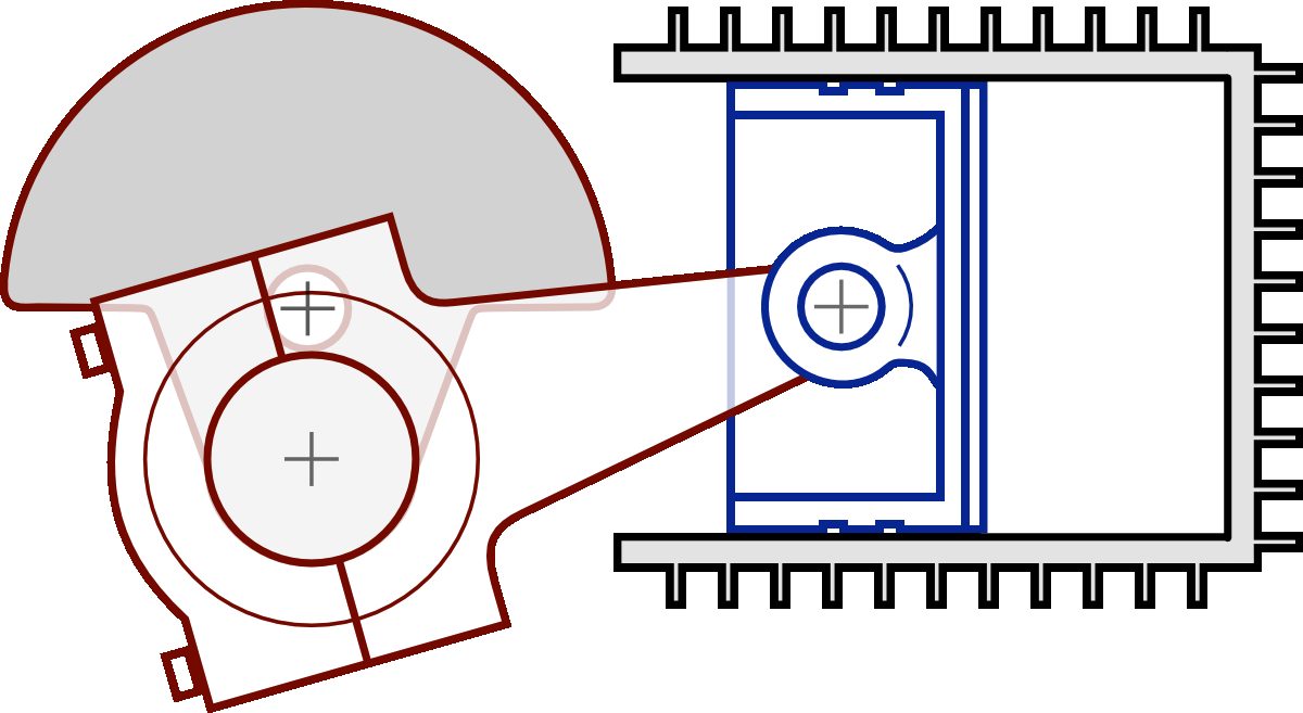
Figure 2.20:Cross-sectional diagram of a small piston air compressor. The intake and exhaust valves are not shown.

Exercise 2.5

Cycle of a Gasoline Engine We want to study the operation of a four-cylinder gasoline engine (figure 2.21). Like all reciprocating heat engines, it supplies work by varying the pressure and volume of small amounts of air trapped in its cylinders. Here, we simplify the details of its operation to reduce it to the ideal case, where all processes are reversible. The engine has a displacement of $1.1 L$ ; it is equipped with four cylinders of diameter $7 cm$ and has a compression ratio (ratio between maximum and minimum volumes in a cylinder) of 7.9. Air enters the engine under atmospheric conditions $(14.5 psi$ or $1 bar, 0.84 m^{3}kg^{-1})$ . We can describe a cycle inside a cylinder with the following four steps: From A to B the air is adiabatically compressed from the bottom dead center to the top dead center. During this process, we know that its properties are related by the relation $p v^{k_{1}}= k_{2}$ . At B, the pressure has reached $246.1 psi (16.97 bar)$ . From B to C it is heated at constant volume (as if the piston were stationary) until the pressure reaches $1087.8 psi (75 bar)$ . By measuring temperature, it is found that its specific internal energy increases by $1543.3 kJ kg^{-1}$ . From C to D the air is adiabatically expanded from the top dead center to the bottom dead center. Its properties are related by the relation $p v^{k_{1}}= k_{3}$ . From D to A it is cooled at constant volume (as if the piston were stationary) until it returns to its state at A. (In practice, this cooling phase takes place outside the engine, in the atmosphere. However, it can be modeled this way without introducing errors.) 1. Draw the processes undergone by the air qualitatively on a pressure-volume diagram. 2. What is the mass of air present in a cylinder? hint: $V_{\mathrm{displacement}}= 4(V_{\max. \mathrm{cylinder}}- V_{\min. \mathrm{cylinder}}) = 4(V_{\mathrm{bottom} \mathrm{dead} \mathrm{center}}- V_{\mathrm{top} \mathrm{dead} \mathrm{center}})$ 3. What is the specific work done to the air during compression (from A to B)? 4. What is the specific heat received by the air during combustion (from B to C)? 5. What is the specific work done by the air during expansion (from C to D)? 6. What is the specific heat transferred away from the air during the cooling phase? 7. What is the engine efficiency, that is, the ratio of the net work output during the cycle to the heat input during combustion? 8. How many cycles must be performed each second for the engine to produce a power of $80 hp (58.84 kW)$ ? Photo CC-by-sa by Commons User:Mj-bird

Answer

$2) V_{\mathrm{A}}= 3.149 \times 10^{-4}m^{3}; \mathrm{so} m_{\mathrm{A}}= \frac{V_{\mathrm{A}}}{v_{\mathrm{A}}} = 3.748 \times 10^{-4}kg$ 3) $k_{1}= 1.3699$ and $k_{2}= 7.8753 \times 10^{4}u.$ si; so $w_{\mathrm{A}\rightarrow \mathrm{B}}= -k_{2}[\frac{1}{-k_{1}+1} v^{-k_{1}+1}]^{v_{\mathrm{B}}}_{v_{\mathrm{A}}}= +260.7kJkg^{-1}.$ 4) $q_{\mathrm{B}\rightarrow \mathrm{C}}= \Delta u-w_{\mathrm{B}\rightarrow \mathrm{C}}= \Delta u-0 = +1543.3 kJ kg^{-1}$ 5) $w_{\mathrm{C}\rightarrow \mathrm{D}}= -k_{3}[\frac{1}{-k_{1}+1} v^{-k_{1}+1}]^{v_{\mathrm{D}}}_{v_{\mathrm{C}}}= - \frac{k_{3}}{k_{2}} w_{\mathrm{A}\rightarrow \mathrm{B}}= - \frac{p_{\mathrm{C}}}{p_{\mathrm{B}}} w_{\mathrm{A}\rightarrow \mathrm{B}}= -1152.2kJkg^{-1}$ 6) $q_{\mathrm{D}\rightarrow \mathrm{A}}= -w_{\mathrm{A}\rightarrow \mathrm{B}}- q_{\mathrm{B}\rightarrow \mathrm{C}}- w_{\mathrm{C}\rightarrow \mathrm{D}}= -651.8 kJ kg^{-1}$ 7) $\eta _{\mathrm{engine}}= \left|\frac{w_{\mathrm{A}\rightarrow \mathrm{B}}+w_{\mathrm{C}\rightarrow \mathrm{D}}}{q_{\mathrm{B}\rightarrow \mathrm{C}}}\right| = 57.8\%$ (very honorable) 8) $f = \frac{\dot{W}_{\mathrm{engine}}}{m_{\mathrm{A}}(w_{\mathrm{A}\rightarrow \mathrm{B}}+w_{\mathrm{C}\rightarrow \mathrm{D}})} = 176.1 Hz$ (176 combustions per second), so approximately 5300 rotations per minute with a four-stroke, four-cylinder engine.

Figure 2.21:Cutaway view of pistons and cylinders of an automobile engine.

Exercise 2.6

Work in a Diesel Engine We are studying the operation of a four-cylinder reciprocating engine by modeling its operation in the most favorable case, in other words, with very slow (perfectly reversible) processes. Inside the engine block schematized in figure 2.22, four pistons linked to the engine shaft by a crankshaft (not shown) are in motion. The process is different in each cylinder: Cylinder A: compression (the air remains trapped in the cylinder). The air compression starts at 0.8 bar and its properties are related by the equation $pV^{1.3}= k_{1}$ . Cylinder B: intake. Air is taken in at constant pressure of 0.8 bar. Cylinder C: exhaust. Air is expelled at constant pressure of 1.1 bar. Cylinder D: expansion. The high-pressure, high-temperature air is trapped in the cylinder; its properties are also related by the equation $pV^{1.3}= k_{2}$ . Diagram CC-by-sa Olivier Cleynen Of course, the role of each cylinder changes twice per revolution. Here, we are studying the work transfers over one half revolution. Even though cylinders B and C are not closed systems, for the purposes of this problem, we can model their processes as if they were, without introducing errors. The atmospheric conditions are 1 bar and $1.225 kg m^{-3}$ . The engine displacement is $1.5 L$ and the compression ratio (that is, the ratio of the minimum to maximum volumes within each cylinder) is 22. 1. Draw the process in each of the cylinders on the same pressure-volume diagram, qualitatively. 2. What is the energy required to move cylinders B and C? 3. What is the energy received by the gas in cylinder A? We want the engine to deliver a power of $30 kW$ at a speed of $2000 revolutions/\min$ . Its mechanical losses are around $15 \%$ . 4. What is the work that must be done by cylinder D during expansion? 5. What should be the pressure generated by combustion in cylinder D, so that the expansion may release enough energy to operate the engine?

Answer

$W_{\mathrm{cyl}.\,\mathrm{B}}= -p_{\mathrm{B}}[V]_{V_{\mathrm{min}}}^{V_{\mathrm{max}}}= -p_{\mathrm{B}}\left(\frac{V_{\mathrm{displacement}}}{4}\right) = -30\,\mathrm{J}$ ; $W_{\mathrm{cyl}.\,\mathrm{C}}= +41.3\,\mathrm{J}$
$V_{\mathrm{A}1}= \frac{22}{21\times 4}V_{\mathrm{swept}}= 3.9286 \times 10^{-4}\,\mathrm{m}^{3}$ and $V_{\mathrm{A}2}= \frac{V_{\mathrm{A}1}}{22} = 1.7857 \times 10^{-5}\,\mathrm{m}^{3}$ . So, $k_{1}= 2.9895\,\mathrm{u.si}$ , and finally $W_{\mathrm{cyl}.\,\mathrm{A}}= \frac{k_{1}}{0.3} (V_{\mathrm{A}2}^{-0.3}- V_{\mathrm{A}1}^{-0.3}) = +160\,\mathrm{J}$ . $4)\;\dot{n} = 2000\,\mathrm{rpm} = 33.3\,\mathrm{rps}$ : there are therefore 66.7 processes per second $(f = 66.7\,\mathrm{Hz})$ . We obtain $W_{4\,\mathrm{cylinders}}= \frac{1}{f}\frac{1}{\eta_{\mathrm{mech}}}\dot{W}_{\mathrm{engine}}$ ; and finally $W_{\mathrm{cyl}.\,\mathrm{D}}= W_{4\,\mathrm{cylinders}}-W_{\mathrm{cyl}.\,\mathrm{A}}-W_{\mathrm{cyl}.\,\mathrm{B}}-W_{\mathrm{cyl}.\,\mathrm{C}}= -700.7\,\mathrm{J}$ .
We calculate $k_{2}$ based on $W_{\mathrm{cyl}.\,\mathrm{D}}$ , and we obtain $p_{\mathrm{D}1}= 194.8\,\mathrm{bar} = 2825\,\mathrm{psi}$ .

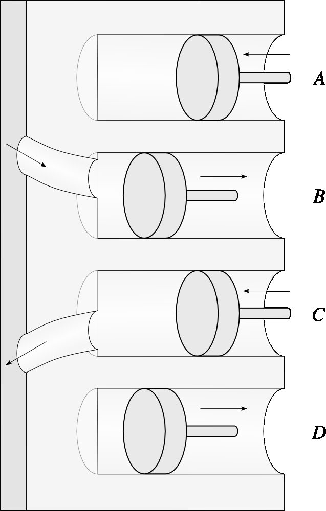
Figure 2.22:Schematic representation of the operation of a four-cylinder engine. Pistons A and C are going up, and pistons B and D are going down. They are all connected to the same motor shaft, not shown here.

Exercise 2.7

Taking Heat From Where it is Cold A student is conducting an experiment with a bit of air in a cylinder, controlling its volume with a piston. The goal is to extract heat from the outside, where the temperature is low, in order to reject it inside the room. The mass of air trapped in the cylinder is $6 \times 10^{-3}kg$ . Initially, the air in the cylinder occupies a volume of $0.5 L (0.132 US gal)$ . The pressure and temperature are room conditions $(1 bar$ ; $18^{\circ}C$ or $64.4 ^{\circ} F)$ . From A to B The student isolates the cylinder well with a thermal insulator, and slowly expands the gas by increasing its volume to $4.5 L (1.189 US gal)$ . We know that during this type of expansion, pressure and volume are related by the equation $pv^{1.4}= k_{2}$ where $k_{2}$ is a constant (we will see where this relationship comes from and learn how to calculate the temperature $T_{\mathrm{B}}$ in chapter 4). The gas temperature drops dramatically during the expansion: at B, the thermometer finally reads $T_{\mathrm{B}}= 121 K$ . From B to C The student ensures the cylinder volume remains constant by mechanically locking the piston, removes the thermal insulator, and places the cylinder outside the building (outside temperature: $-5^{\circ}C$ or $23 ^{\circ} F)$ . The gas temperature and pressure slowly rise. From C to A When the pressure reaches 1 bar precisely, the cylinder air temperature is indicated as $T_{\mathrm{C}}= 262 K$ . The student wishes to return to the initial conditions (by reducing the volume to the initial volume) while keeping the pressure constant at 1 bar. 1. Sketch the process on a pressure-volume diagram. 2. Show that during a reversible process undergone by a closed system whose properties are related by a relation of the form $pv^{k_{1}}= k_{2}$ (where $k_{1}\neq 1$ and $k_{2}$ are constants), the specific work done is: $w_{\mathrm{A}\rightarrow \mathrm{B}}= \frac{p_{\mathrm{B}}v_{\mathrm{B}}- p_{\mathrm{A}}v_{\mathrm{A}}}{k_{1}- 1}$ 3. What is the work done by the gas during the expansion? 4. The thermal capacity of air when its volume is fixed is $718 J kg^{-1}K^{-1}$ . How much heat was transferred to or from the outside air? 5. How much work will be needed to perform the C $\rightarrow$ A return at constant pressure? 6. Over the entire cycle, will the student have done or received work? 7. [difficult question] The return path at constant pressure requires heat transfer. In which direction and to what extent? Why can’t (unfortunately) this transfer be entirely done inside the building?

Answer

After obtaining $p_{\mathrm{B}}= 4.61 \times 10^{-2}bar$ , we calculate $W_{\mathrm{A}\rightarrow \mathrm{B}}= \frac{p_{\mathrm{B}}V_{\mathrm{B}}-p_{\mathrm{A}}V_{\mathrm{A}}}{k_{1}-1} = -73.14 J$ .
$Q_{\mathrm{B}\rightarrow \mathrm{C}}= mc_{v}\Delta T = +607.4 J$
$W_{\mathrm{C}\rightarrow \mathrm{A}}= +400 J$ (easy!)
$W_{\mathrm{cycle}}= +326.86 J$ , so work done by the student.
$Q_{\mathrm{C}\rightarrow \mathrm{A}}= -934.26 J$
It is a matter of temperature... Engineering Thermodynamics by Olivier Cleynen