6. Thermodynamic Cycles - Engineering Thermodynamics

Thermodynamic Cycles

A Foray into the Sorcery of Heat Mechanics

Introduction¶

Thanks to chapters 4 and 5, we have learned to quantify energy in fluids based on their properties. We will now use these fluids in machines to convert heat into work, and work into heat. In this chapter 6 (thermodynamic

cycles), we aim to formalize the concept of a cycle, addressing two questions:

• How do engines, refrigerators, and heat pumps work?

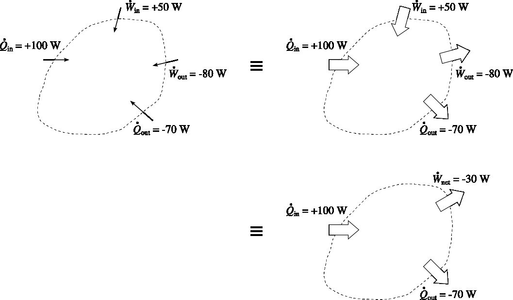
• How is their efficiency quantified?

6.1 Graphical Conventions¶

We start by agreeing on some graphical and notation conventions, which are summarized in figure 6.1.

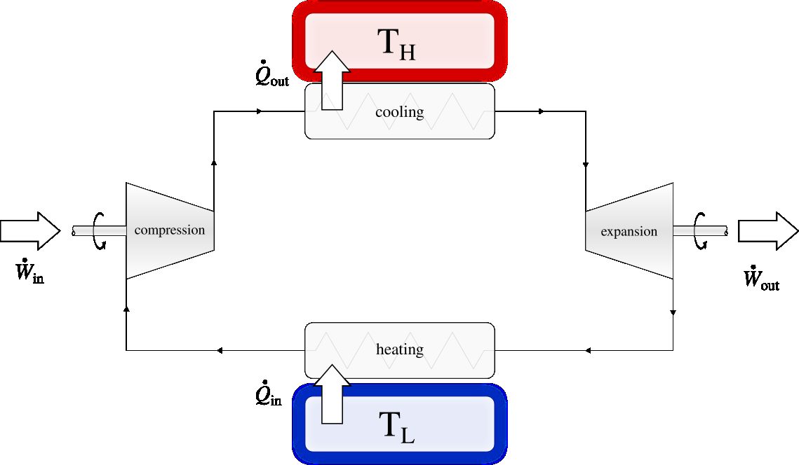
Figure 6.1:New graphical and notation conventions for energy transfers. The white arrows are oriented according to the physical direction of the transfers; The algebraic sum of all the work received and carried out is represented by a single transfer named *net work*.

Diagram CC-0 Olivier Cleynen

We use large white arrows to represent the physical direction of transfers. We do not change our sign convention (transfers are positive when directed toward the system and negative when coming from it), but only the graphical convention for their orientation, in order to make the visualization of transfers in machines more intuitive.

The algebraic sum of the work $W_{\mathrm{in}}$ received by a machine and $W_{\mathrm{out}}$ it supplies is named the net work $W_{\mathrm{net}}$ . The net work can be positive (done onto the the machine from external sources) or negative (done by the machine to an external receiver), depending on the application.

W_{\mathrm{net}}\equiv W_{\mathrm{in}}+ W_{\mathrm{out}}

(1)

W_{\mathrm{net}}\equiv \dot{W}_{\mathrm{in}}+\dot{W}_{\mathrm{out}}

(2)

w_{\mathrm{net}}\equiv w_{\mathrm{in}}+ w_{\mathrm{out}}

(6/1)

We define the net heat in the same way:

Q_{\mathrm{net}}\equiv Q_{\mathrm{in}}+ Q_{\mathrm{out}}

(3)

Q_{\mathrm{net}}\equiv \dot{Q}_{\mathrm{in}}+\dot{Q}_{\mathrm{out}}

(4)

q_{\mathrm{net}}\equiv q_{\mathrm{in}}+ q_{\mathrm{out}}

(6/2)

Therefore, for example, a car’s engine sees a positive net heat transfer (reception) and a negative net work (supplied to the gearbox).

6.2 Transforming Heat and Work¶

6.2.1 Building thermodynamic cycles¶

We want to compare different ways of transforming work and heat. For these comparisons to be valid, we must always take into account all the processes undergone by the fluid until it returns to its initial state.

For example, it is easy to cool a room with a compressed air bottle (simply make the fluid work during its expansion to lower its temperature); but if we want to continuously cool the room, then we also need to consider the energy required to return the air to the bottle, at its initial pressure and temperature, at the end of the process.

A second example is that of a car engine, which releases heat carried by the exhaust gases. In order to account for this lost energy, we count the heat that would need to be removed from the gases in order to bring them back to the engine’s inlet temperature. This imaginary cooling takes place outside the engine in practice, but from a thermodynamic standpoint, it is an integral part of the energy transformation process.

Therefore, every time we analyze the operation of a thermodynamic machine, we will make sure to continue the fluid processes until it returns to its initial state (same temperature, same pressure, same internal energy, etc.). We then say that it has completed a thermodynamic cycle (§2.3).

6.2.2 Producing work with heat¶

Let us start by compressing a fluid: we increase its pressure and reduce its specific volume, which requires a certain amount of work. After that, we heat up this fluid: its pressure and volume tend to increase. By expanding the fluid back to its initial pressure, we will recover more work than what we initially invested. Finally, in order to bring the fluid back to its initial state, it needs to be cooled down.

In the end, the fluid has done more work when it was expended than was done onto it when it was compressed. Over a cycle, it will thus have produced work and absorbed heat (part of which it transformed). This is the operating principle of an engine.

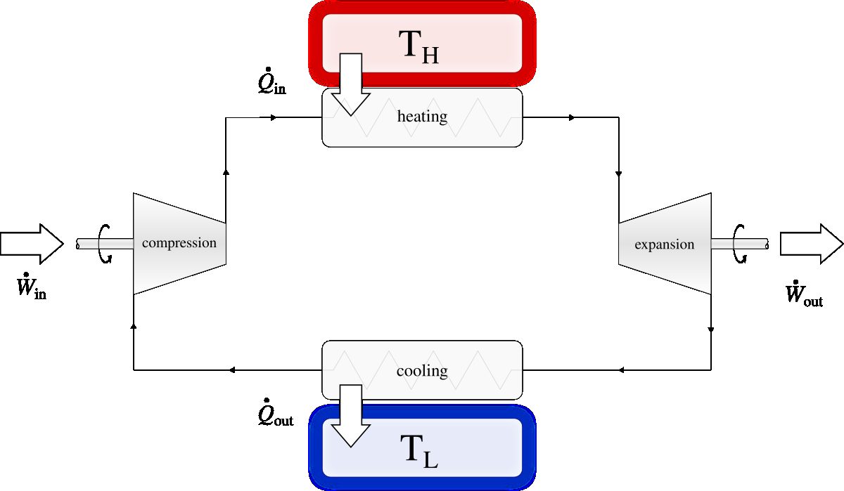
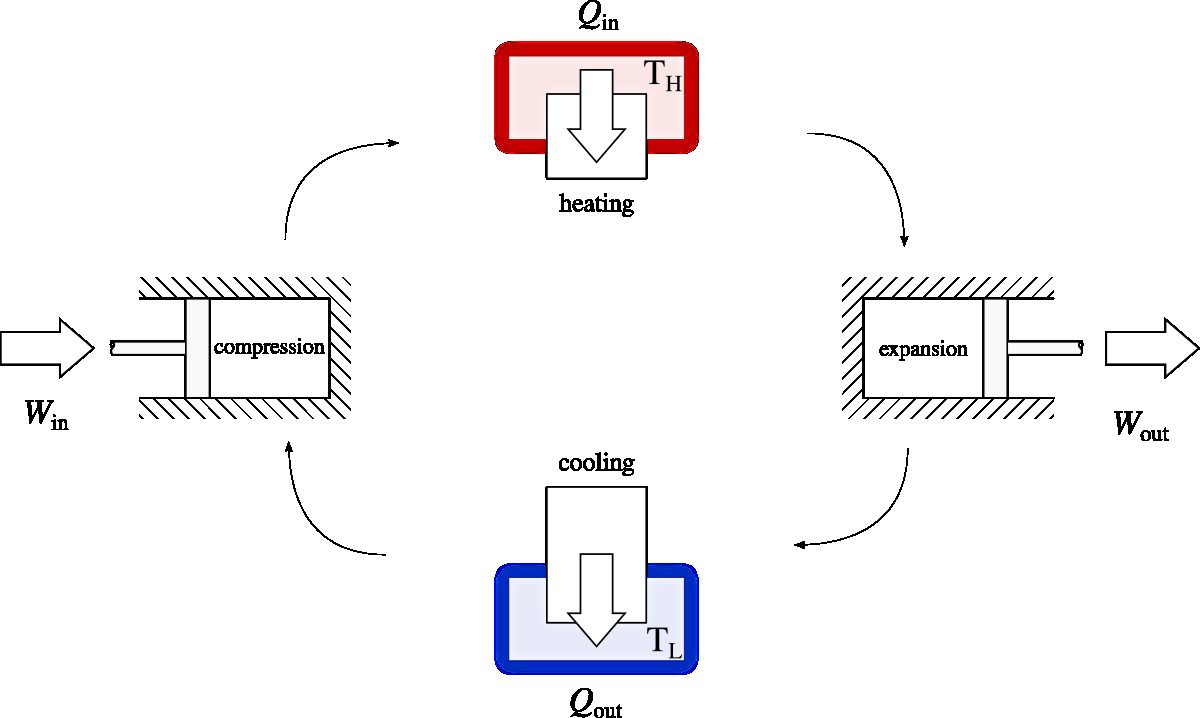
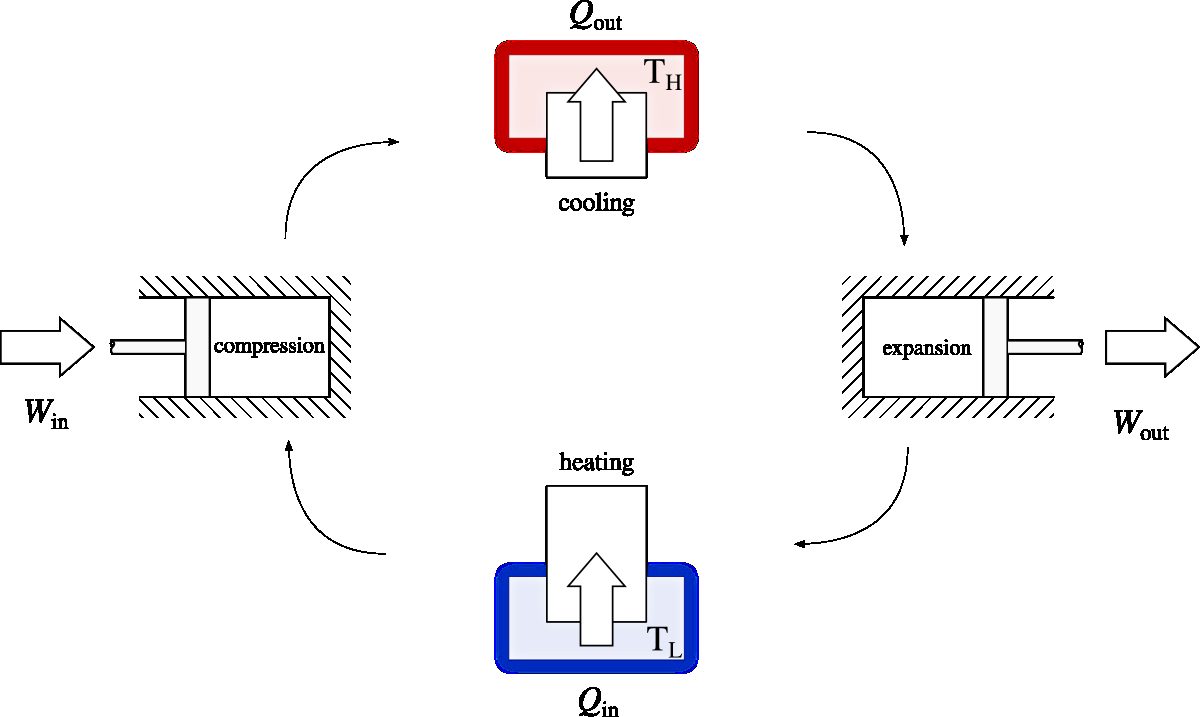
There are infinitely many possible cycles to perform this process, but they all involve at least four energy transfers: compression, heating, expansion, and cooling. We can separate these processes in space, as shown in figure 6.3, or in time, as illustrated in figure 6.2. Depending on technological and practical constraints, some of these transfers may be performed simultaneously.

Engine thermodynamic cycle. The fluid absorbs heat supplied at high temperature $T_{H}$. The compression power is lower than the expansion power: the net power in the form of work$\dot{W}_{\mathrm{net}}=\dot{W}_{\mathrm{in}}+\dot{W}_{\mathrm{out}}$ is negative. — Figure 6.2:Engine thermodynamic cycle. The fluid absorbs heat supplied at high temperature $T_{H}$ . The compression power is lower than the expansion power: the net power in the form of work $\dot{W}_{\mathrm{net}}=\dot{W}_{\mathrm{in}}+\dot{W}_{\mathrm{out}}$ is negative.

Diagram CC-0 Olivier Cleynen

Engine thermodynamic cycle carried out by separating the stages in time (rather than in space as shown in figure 6.2). The fluid is heated by a high-temperature heat source $T_{H}$. The net work $W_{\mathrm{net}}= W_{\mathrm{in}}+ W_{\mathrm{out}}$ is negative. — Figure 6.3:Engine thermodynamic cycle carried out by separating the stages in time (rather than in space as shown in figure 6.2). The fluid is heated by a high-temperature heat source $T_{H}$ . The net work $W_{\mathrm{net}}= W_{\mathrm{in}}+ W_{\mathrm{out}}$ is negative.

Diagram CC-0 Olivier Cleynen

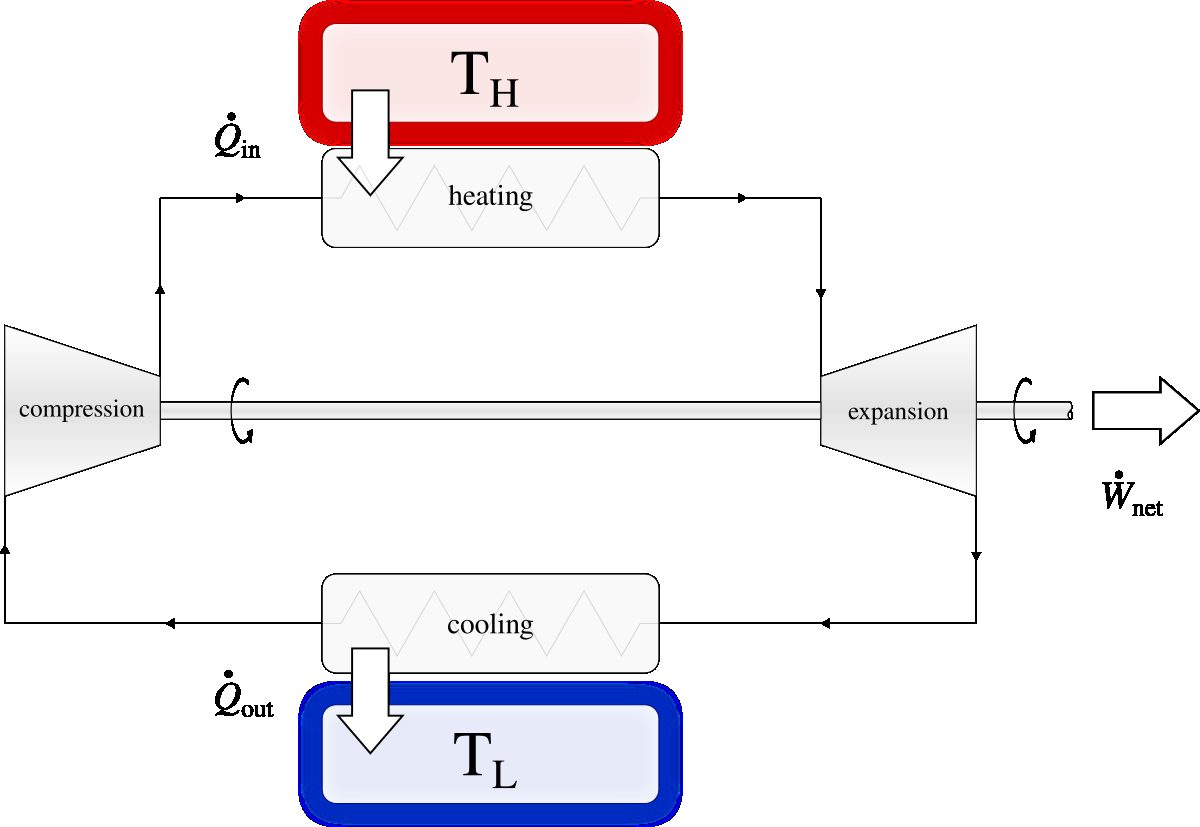
It is possible to mechanically link the sections that receive and supply energy in the form of work. In the case where the fluid circulates continuously, the compressor and the turbine can be connected by the same shaft, as shown in figure 6.4. In the case where the processes are separated in time, such as in an internal combustion engine, the processes can be linked by performing multiple offset cycles simultaneously (with multiple cylinders) or by storing energy in a flywheel. The engine then does not receive external work, and the resulting output is a power $\dot{W}_{\mathrm{net}}$ .

An engine thermodynamic cycle in which the compressor and the turbine are mechanically coupled. Since the turbine supplies a power$\dot{W}_{\mathrm{out}}$ greater than that absorbed by the compressor $(\dot{W}_{\mathrm{in}})$, it is able to not only drive the compressor but also to provide an excess$\dot{W}_{\mathrm{net}}$ sent outside of the engine. — Figure 6.4:An engine thermodynamic cycle in which the compressor and the turbine are mechanically coupled. Since the turbine supplies a power $\dot{W}_{\mathrm{out}}$ greater than that absorbed by the compressor $(\dot{W}_{\mathrm{in}})$ , it is able to not only drive the compressor but also to provide an excess $\dot{W}_{\mathrm{net}}$ sent outside of the engine.

Diagram CC-0 Olivier Cleynen

6.2.3 Extracting heat with work¶

When work is done on a fluid, its temperature tends to rise (with a brief exception for liquid/vapors between their saturation points) and it can thus supply heat to a body that was initially at a higher temperature (“hotter”) than itself.

Conversely, when a fluid is expanded, its temperature tends to decrease and it can thus absorb heat from a body that was initially “colder” than itself.

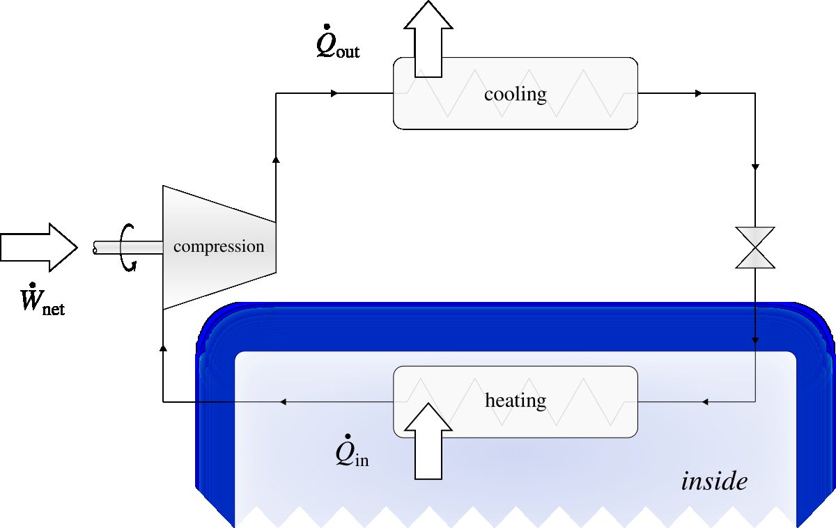
By performing these steps one after the other, we obtain a refrigeration cycle: a machine capable of extracting heat at low temperature and rejecting it at high temperature. Such a cycle is depicted in figures 6.6 (stages separated in space) and 6.5 (stages separated in time).

Careful examination of these two figures will reveal a major surprise: they are exactly the same arrangement as for an engine! The only difference lies in the operating temperatures. The temperature reached during compression must be higher than the high temperature $T_{H}$ , and the temperature reached during expansion must be lower than the low temperature $T_{L}$ . Unless these conditions are met, the heat transfers will occur in the wrong direction.

In a refrigeration cycle, the fluid has a larger volume when compressed (after having being heated) than when expanded (after having being cooled): this time, the compression requires more power than the expansion. The net power $\dot{W}_{\mathrm{net}}$ in the form of work is therefore positive, meaning that the machine must be powered by an external source of work.

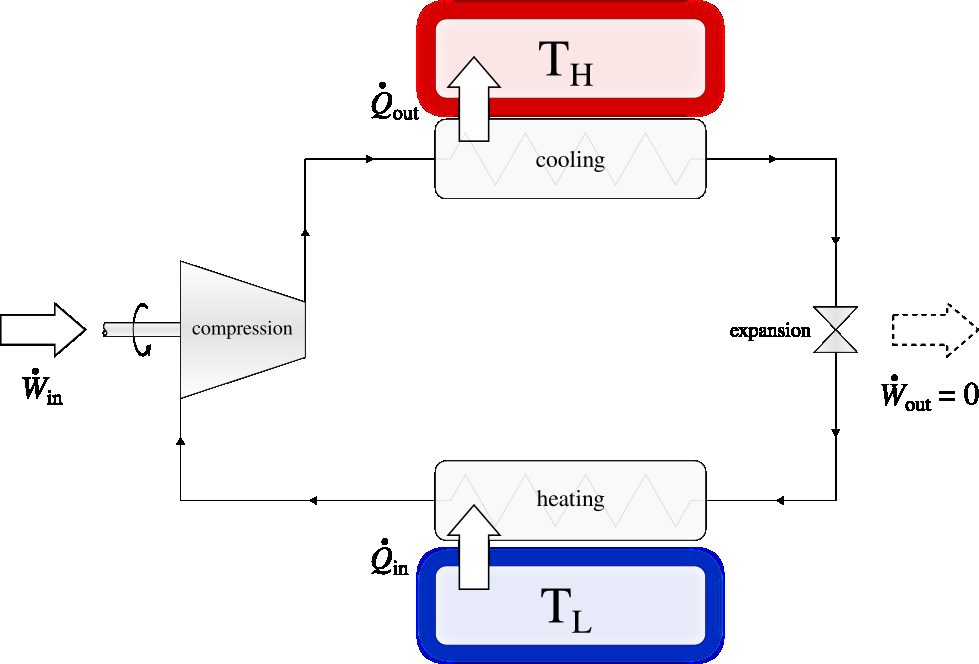
In practice in refrigeration systems, a trick is often used to lower the temperature: instead of a turbine, a simple valve (sometimes called a throttling valve) is used. In this component without moving parts, the fluid does not do work (therefore the power to be supplied to the machine is increased),

A refrigeration cycle, for use in refrigerators, air conditioners, and heat pumps. A power$\dot{Q}_{\mathrm{in}}$ in the form of heat is absorbed at low temperature (the fluid is then heated) while a power$\dot{Q}_{\mathrm{out}}$ is rejected at high temperature (the fluid is then cooled). — Figure 6.5:A refrigeration cycle, for use in refrigerators, air conditioners, and heat pumps. A power $\dot{Q}_{\mathrm{in}}$ in the form of heat is absorbed at low temperature (the fluid is then heated) while a power $\dot{Q}_{\mathrm{out}}$ is rejected at high temperature (the fluid is then cooled).

Diagram CC-0 Olivier Cleynen

Figure 6.6:A refrigeration cycle carried out by separating the stages in time (rather than in space as shown in figure 6.5)

Diagram CC-0 Olivier Cleynen but it is much simpler to manufacture and use. This modification is depicted in figure 6.7.

The throttle valve, in thermodynamic terms, allows for a completely irreversible expansion, increasing the volume and reducing the pressure without extracting work. If a perfect gas were used, this would have no effect on the temperature (as in the experiments of Joule and Gay-Lussac studied in §4.3.2 p. 90) and therefore no interest; but when liquids/vapors are used, the throttling expansion is a technologically simple way to lower the temperature.

Figure 6.7:A modified refrigeration cycle using a throttling valve. When using liquids/vapors, it is possible to avoid extracting work during expansion. The use of a simple valve is sufficient to lower the temperature of the fluid.

Diagram CC-0 Olivier Cleynen

Refrigeration cycles have two main types of applications:

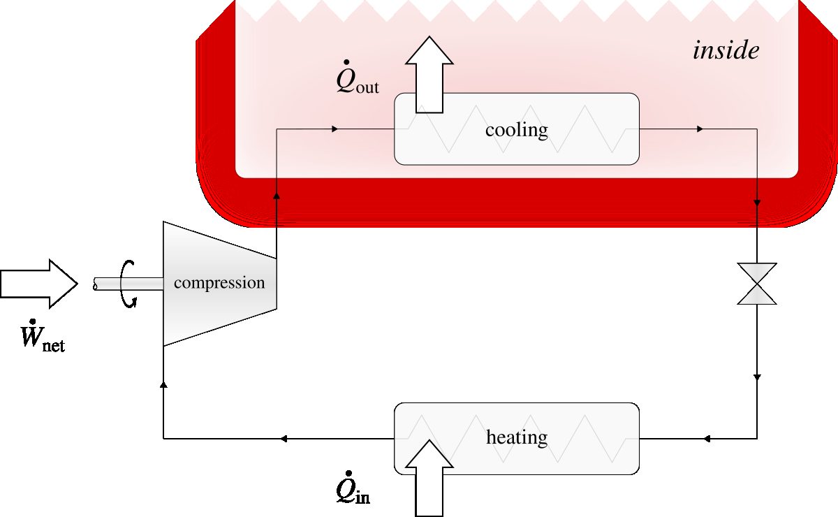
Heat pumps (figure 6.8) are arranged to reject heat to a high-temperature body, most often a building;

Refrigerators and air conditioners (figure 6.9) are arranged to extract heat from a low-temperature body (a cold enclosure).

Figure 6.8:Arrangement of a heat pump. The machine is configured to reject heat inside (where the temperature is higher) which it extracts from outside (where the temperature is lower).

Diagram CC-0 Olivier Cleynen

Figure 6.9:Arrangement of a refrigerator or air conditioner. The machine is configured to reject heat outside (where the temperature is higher) which it extracts from the inside (where the temperature is lower). This is exactly the same machine as in figure 6.8.

Diagram CC-0 Olivier Cleynen

In these two types of applications, it is exactly the same machine, operating with the same cycle. The only difference concerns the internal/external arrangement of the components: a heat pump is nothing more than a refrigerator positioned to “cool the outside”.

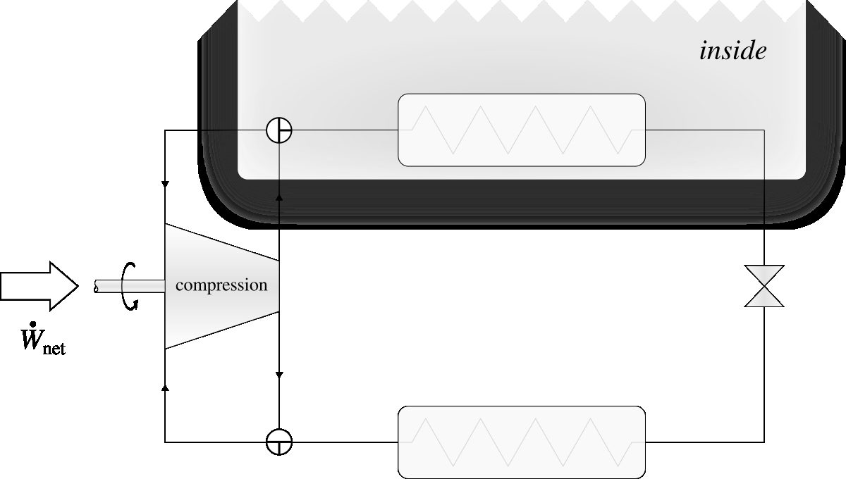
The similarity between an air conditioner and a heat pump allows these two functions to be performed by a single machine, which is then referred to as reversible in the industry. In thermodynamics, the word “reversible” has a different meaning, as we will see in chapter 7 (the second law), and so we will call this kind of machine bidirectional here. Depending on the needs, the direction of fluid flow is reversed, which causes the inversion of heat transfers. This type of machine is shown in figure 6.10.

Figure 6.10:Layout of a bidirectional (commonly called “reversible”) air conditioner. By rotating both valves 90 degrees counterclockwise, the function changes from a heat pump to an air conditioner.

Diagram CC-0 Olivier Cleynen

6.3 Cycle Efficiency¶

6.3.1 A basic formula¶

The efficiency^[1] $\eta$ of a thermodynamic machine compares the useful transfer or transformation it performs with the energy cost it incurs. We will adopt the following principle definition:

\eta \equiv \left|\frac{\mathrm{useful} \mathrm{transfer}}{\mathrm{energy} \mathrm{expenditure}}\right|

(6/3)

By convention, the efficiency is always expressed as a positive number; thus we use an absolute value in equation 6/3. For each of the three types of thermodynamic machine, we will define and quantify this “useful transfer” and this “energy expenditure”.

6.3.2 Efficiency of an engine¶

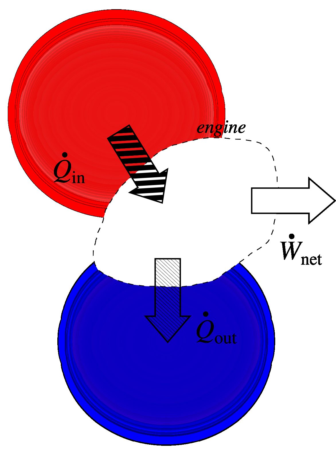
The function of a thermal engine, like those found on board road vehicles or in power plants, is to supply work, meaning a negative quantity $\dot{W}_{\mathrm{net}}$ (figure 6.11). The expense incurred to generate this work is the heat it receives, namely the quantity $\dot{Q}_{\mathrm{in}}$ (usually originating from the combustion of fuel or the fission of atomic nuclei).

Energy transfers associated with an engine. We aim to obtain a large transfer$\dot{W}_{\mathrm{net}}$ (result) from the transfer$\dot{Q}_{\mathrm{in}}$ (cost). The rejection$\dot{Q}_{\mathrm{out}}$ is undesirable. — Figure 6.11:Energy transfers associated with an engine. We aim to obtain a large transfer $\dot{W}_{\mathrm{net}}$ (result) from the transfer $\dot{Q}_{\mathrm{in}}$ (cost). The rejection $\dot{Q}_{\mathrm{out}}$ is undesirable.

Diagram CC-0 Olivier Cleynen

According to definition 6/3, the efficiency $\eta _{\mathrm{engine}}$ of the thermal engine is therefore:

\eta _{\mathrm{engine}}\equiv \left|\frac{\dot{W}_{\mathrm{net}}}{\dot{Q}_{\mathrm{in}}}\right|

(6/4)

Example 6.1

A car engine receives $100 kW$ in the form of heat from gasoline combustion; it supplies $55 kW$ as work at the transmission shaft. What is its efficiency?

The efficiency is $\eta _{\mathrm{engine}}= \left|\frac{\dot{W}_{\mathrm{net}}}{\dot{Q}_{\mathrm{in}}}\right| = \left|\frac{-55 \times 10^{3}}{+100 \times 10^{3}}\right| = 0.55 = 55 \%$ .

This engine rejects $\dot{Q}_{\mathrm{out}}= -\dot{W}_{\mathrm{net}}-\dot{Q}_{\mathrm{in}}= -(-55 \times 10^{3}) - 100 \times 10^{3}= -45 kW$ as heat. Most of this energy is carried away with the exhaust gases.

Since one must always supply at least as much heat $\dot{Q}_{\mathrm{in}}$ as the engine outputs in work $\dot{W}_{\mathrm{net}}$ , the efficiency of an engine will always necessarily be less than 1.

The net power $\dot{W}_{\mathrm{net}}$ in the form of work can be expressed in terms of other energy transfers, as follows:

W_{\mathrm{net}}=\dot{W}_{\mathrm{in}}+\dot{W}_{\mathrm{out}}= -Q\dot{} _{\mathrm{in}}-\dot{Q}_{\mathrm{out}}

(5)

\eta _{\mathrm{engine}}= 1 - \left|\frac{\dot{Q}_{\mathrm{out}}}{\dot{Q}_{\mathrm{in}}}\right|

(6/5)

This equation 6/5 will be very useful in the next chapter (§7.5.1 p. 195), where we will want to relate the heat transfers $\dot{Q}_{\mathrm{in}}$ and $\dot{Q}_{\mathrm{out}}$ to the temperatures at which they occur.

6.3.3 Efficiency of a refrigerator or air conditioner¶

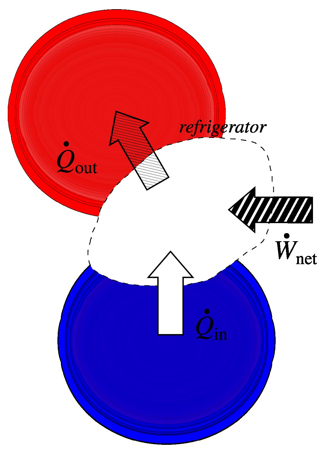
The function of a refrigerator or an air conditioner is to extract heat, and thus to generate a positive power $\dot{Q}_{\mathrm{in}}$ (heat extracted every second from the compartment to be cooled). This transfer (figure 6.12) is made possible by supplying work to the refrigerator, $\dot{W}_{\mathrm{net}}$ , an “expense” that must be positive, too.

According to the definition 6/3, the efficiency of a refrigerator or an air conditioner, also called the coefficient of performance cop $_{\mathrm{refrigeration}}$ , is therefore:

\eta _{\mathrm{refrigerator}}= \eta _{\mathrm{air} \mathrm{conditioner}}\equiv \left|\frac{\dot{Q}_{\mathrm{in}}}{\dot{W}_{\mathrm{net}}}\right|

(6/6)

Energy transfers associated with a refrigerator or an air conditioner. We aim to obtain a large transfer$\dot{Q}_{\mathrm{in}}$ (result) from the transfer$\dot{W}_{\mathrm{net}}$ (cost). — Figure 6.12:Energy transfers associated with a refrigerator or an air conditioner. We aim to obtain a large transfer $\dot{Q}_{\mathrm{in}}$ (result) from the transfer $\dot{W}_{\mathrm{net}}$ (cost).

Diagram CC-0 Olivier Cleynen

Example 6.2

A refrigerator receives an electrical power of $100 W$ ; it extracts heat from the cold chamber with a power of $120 W$ . What is its efficiency?

The efficiency (or cop) is $\eta _{\mathrm{refrigerator}}= \left|\frac{\dot{Q}_{\mathrm{in}}}{\dot{W}_{\mathrm{net}}}\right| = \left|\frac{+120}{+100}\right| = 1.2 = 120 \%$ .

This refrigerator rejects $\dot{Q}_{\mathrm{out}}= -\dot{W}_{\mathrm{net}}-\dot{Q}_{\mathrm{in}}= -100 - 120 = -220 W$ outside of the cold chamber (usually, within the building itself).

Household refrigerators and air conditioners often have efficiencies greater than 1, but depending on the desired temperatures, the efficiency can indeed be lower.

In order to prepare for the next chapter (§7.5.2 p. 196), and while paying attention to the pitfalls associated with the use of absolute values, we can express this efficiency in terms of heat transfers only:

\eta _{\mathrm{refrigerator}}= \eta _{\mathrm{air} \mathrm{conditioner}}= \frac{1}{\left|\frac{Q_{\mathrm{out}}}{Q_{\mathrm{in}}}\right| - 1}

(6/7)

6.3.4 Efficiency of a heat pump¶

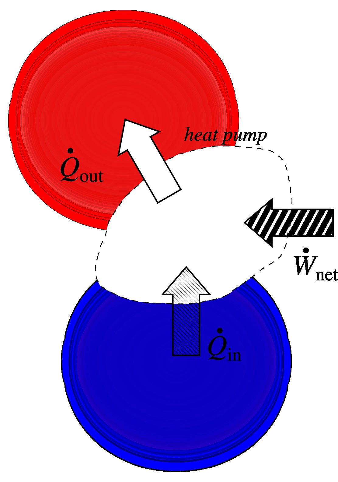
A heat pump operates exactly the same way as an air conditioner. Its function is to generate a transfer $\dot{Q}_{\mathrm{out}}$ to the “hot” section (usually inside a building). This transfer, represented in figure 6.13, is made possible by supplying work to the heat pump, $\dot{W}_{\mathrm{net}}$ , an “expense” that is necessarily positive.

Energy transfers associated with a heat pump. We aim to obtain a large transfer$\dot{Q}_{\mathrm{out}}$ (result) from the transfer$\dot{W}_{\mathrm{net}}$ (cost). — Figure 6.13:Energy transfers associated with a heat pump. We aim to obtain a large transfer $\dot{Q}_{\mathrm{out}}$ (result) from the transfer $\dot{W}_{\mathrm{net}}$ (cost).

Diagram CC-0 Olivier Cleynen

The efficiency $\eta _{\mathrm{heat} \mathrm{pump}}$ of the heat pump, also known as the coefficient of performance cop $_{\mathrm{heat} \mathrm{pump}}$ , is thus defined as:

\eta _{\mathrm{heat} \mathrm{pump}}\equiv \left|\frac{\dot{Q}_{\mathrm{out}}}{\dot{W}_{\mathrm{net}}}\right|

(6/8)

Just as we did for the previous sections, we can express this efficiency in terms of heat flows only:

\eta _{\mathrm{heat} \mathrm{pump}}= \frac{1}{1 - \left|\frac{Q_{\mathrm{in}}}{Q_{\mathrm{out}}}\right|}

(6/9)

6.3.5 On the low performance of machines¶

In all the cases we have studied above, for each cycle, we have included an undesirable transfer. In the engine cycle, some of the energy is wasted in the form of heat rejection $(\dot{Q}_{\mathrm{out}})$ . In refrigeration cycles, work must be supplied $(\dot{W}_{\mathrm{in}})$ to carry out a heat transfer that a priori could have seemed “free” $(\dot{Q}_{\mathrm{out}}$ then being equal to $\dot{Q}_{\mathrm{in}})$ . Engineering students will certainly be indignant about the role played by these losses in this chapter – and about the modest efficiencies achieved by the machines described in the examples. Why are the efficiencies calculated in the examples and in the following problems so low, and more importantly, how can we design cycles with greater efficiency? We take these worries to our heart, and will address them in chapter 7 (the second law).

A Bit of History

the Number of Strokes

Historically, we have learned to transform heat into work by manipulating fixed quantities of fluid trapped in enclaves. These enclaves have always been of cylindrical geometry, which greatly facilitates the manufacture of pistons that exploit the changes in volume of the fluid in order to extract work from it.

When the fluid is water, heat is supplied in a boiler and the steam is then transferred to the cylinder or cylinders in order to be expanded (§9.4). However, at the end of the 19th century, air began to be used, a fluid inside which heat could be directly generated by combustion. The complex process of conducting a separate combustion to heat a metallic boiler which then finally heats the water of the engine was eliminated, along with all the heat and temperature losses it entailed. This was the birth of the internal combustion engine, the development of which was notably driven by the German engineers Nicolaus Otto and Rudolf Diesel (§10.3). Combustion and expansion were now carried out in the same place, directly in the cylinder.

However, in order to achieve internal combustion, a new problem had to be solved: since the oxygen in the air is used, the combustion can only be carried out once. After each combustion, it is therefore essential to expel the reaction products (CO $_{2}$ and H $_{2}$ O primarily) from the cylinder and to reintroduce “fresh” air containing the oxygen O $_{2}$ necessary for breaking the hydrocarbon molecules $\mathrm{C}_{x}$ H $_{y}$ that produce heat. Two different solutions were then adopted.

The most common method dedicates one piston movement to each step: the first one for compression, the second one for expansion (after or during combustion), the third one for exhaust gases expulsion (exhaust), and the last one for admitting fresh air (intake). Engines following this process are called four-stroke (figure 6.14), and they have always been the most widely used.

The second method is bound to offend purists: it performs these four operations in two strokes only. In these engines, part of the gas expansion is used to perform the exhaust, and it is carried out simultaneously with the air intake (figures 6.15 and 6.16). Certainly, none of the four steps can be optimally performed: the compression and expansion phases are only carried out over a portion of the stroke, and the scavenging is necessarily incomplete due to the mixing of fresh and exhaust gases. On the other hand, the combustions are twice as frequent, since there is no need for intake and exhaust strokes during which no thermodynamic operation takes place. Thus, for the same displacement and speed of rotation, two-stroke engines are much more powerful than their four-stroke counterparts, even though they are also significantly less efficient.

Two- and four-stroke engines were developed at the same time, but two-stroke engine development really took off after the Second World War. The refinement by the German engineer Walter Kaaden of an ingenious exhaust system, whose geometry alone increases the airflow escaping during expansions and reduces it during compressions, made the engine very competitive in racing motorcycles; this tuned expansion chamber (figure 6.17) was adopted in many production models.

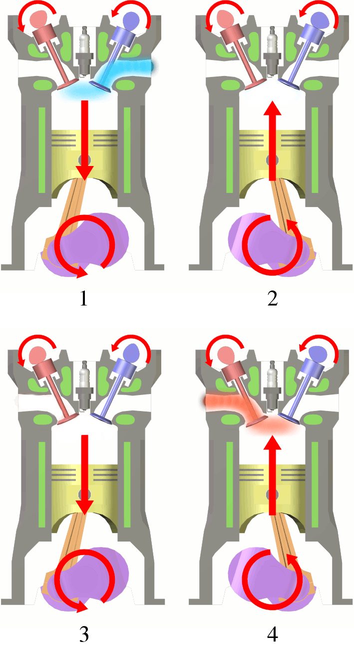
Figure 6.14:The four steps of a four-stroke engine. The piston descends to admit fresh air coming from the right (*intake* stroke, 1); it then rises to increase the air temperature (*compression* stroke, 2); useful work production occurs during a descent (*power* stroke, 3); finally, the air is expelled to the outside during a fourth and last movement (*exhaust* stroke, 4) before starting the cycle again. Most current piston-cylinder engines follow this process.

Diagrams 1 2 3 4 CC-by by Eric Pierce

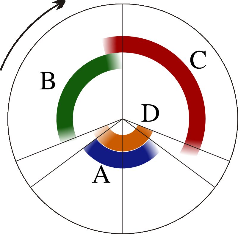
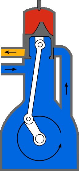
Figure 6.15:Cycle of a two-stroke engine. The four necessary steps for operation are carried out in a single revolution of the crankshaft, that is, two piston movements. Intake (A) occurs during the passage at bottom dead center, compression (B) starts late, and expansion (C) is interrupted to allow scavenging (D) when the piston approaches bottom dead center again.

Diagram derived from a diagram CC-by-sa by Commons User:A7N8X

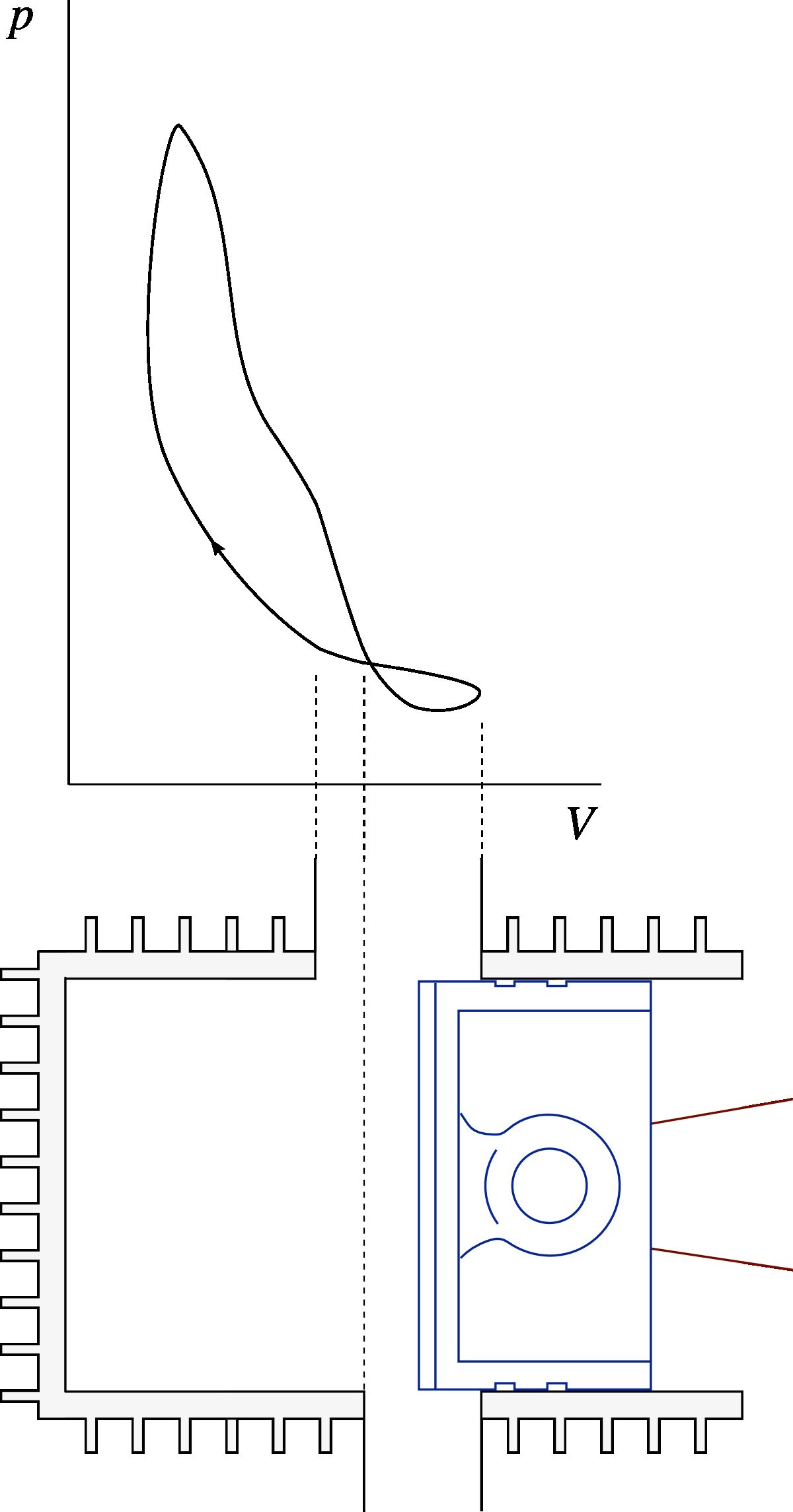
Figure 6.16:Schematic pressure-volume diagram of the cylinder of a two-stroke engine with crankcase intake. It is left to the student to determine which of the two ports (high or low) corresponds to intake and exhaust in the cylinder.

Diagram CC-by-sa by Commons User:Terraflorin & Olivier Cleynen

In parallel, the ideas formulated by the English entrepreneur Joseph Day at the end of the 19th century on the mechanism controlling intake spread widely.

With his ingenious crankcase intake, it is the piston itself that serves as a valve (figure 6.18). The intake air first passes through the crankcase where the crankshaft rotates, then it is slightly compressed by the piston in its downward movement before entering the cylinder. The engine thus operates without any moving valve; lubrication can even be provided simply by injecting oil directly into the intake air.

With these two advantages, the engine found its application wherever constraints of weight, volume, acquisition cost, and maintenance took precedence over efficiency. After powering three million Trabant cars in East Germany, it was adopted on nearly all outdoor portable tools (chainsaws, lawnmowers, etc.). The engine can easily be miniaturized, leaving room for legs on a scooter motorcycle, allowing snowmobiles to start easily, in short, until the 90s, nothing —not even homeowner associations!— seemed to be able to halt its progress.

However, at the beginning of the 21st century, it becomes necessary to give up on these advantages.

One can wearily accept the irritating sound emitted by the two-stroke engine, but its polluting emissions are staggering. Lubrication by oil injection into the intake air causes the atmospheric discharge of smoke, odors, and harmful particles. In addition, the always incomplete scavenging of the cylinder greatly limits the efficiency of combustion and the thermal efficiency. The tightening of regulations controlling emissions gradually forces the replacement of these engines with four-stroke ones or electric systems — whose batteries are often charged with energy from power plants... powered by steam engines. We see that seemingly minor technological decisions can sometimes have consequences on a global scale!

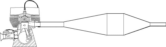
Figure 6.17:Tuned (sometimes called “harmonic”) expansion chamber mounted on a two-stroke engine. Since the flow is unsteady, it is possible to manipulate the pressure exerted by fixed amounts of exhaust gases on the exhaust port when they pass through the chamber. Passing through the expansive part reduces the pressure (thus facilitating scavenging during the piston descent), while passage through the contraction, on the contrary, increases this pressure (thus reducing gas losses during the piston ascent).

Diagram CC-by-sa by Achim Agster

Figure 6.18:Crankcase intake system. The intake air, laden with fuel for combustion and oil for lubricating mechanical parts, first enters the crankcase. It is compressed and then inserted into the cylinder with the sole downward movement of the piston. There is no need for any valve or flap.

Diagram public domain by Commons User:Tomeq183

Problems¶

Air is considered an ideal gas.

$c_{v (\mathrm{air})}= 718 J kg^{-1}K^{-1} \qquad R_{\mathrm{air}}= 287 J kg^{-1}K^{-1}$

$c_{p (\mathrm{air})}= 1005 J kg^{-1}K^{-1} \qquad \gamma _{\mathrm{air}}= 1.4$

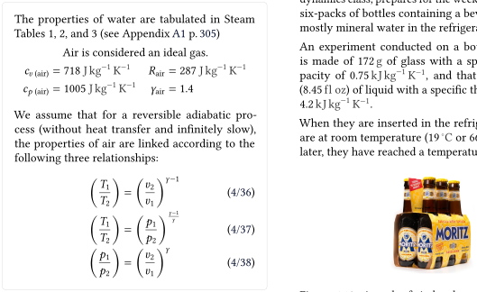
We assume that for a reversible adiabatic process (without heat transfer and infinitely slow), the properties of air are linked according to the following three relationships:

\left(\frac{T_{1}}{T_{2}}\right) = \left(\frac{v_{2}}{v_{1}}\right)^{\gamma -1} \qquad (4/36)

(6)

\left(\frac{T_{1}}{T_{2}}\right) = \left(\frac{p_{1}}{p_{2}}\right)^{\frac{\gamma -1}{\gamma}} \qquad (4/37)

(7)

\left(\frac{p_{1}}{p_{2}}\right) = \left(\frac{v_{2}}{v_{1}}\right)^{\gamma} \qquad (4/38)

(8)

Exercise 6.1

Engine Efficiency The Diesel engine of an excavator has an efficiency of $40\%$ and delivers a continuous power of $60 kW$ (approximately $80 hp$ ). It is powered by fuel with a calorific value of $35 MJ kg^{-1}$ . 1. What is the hourly fuel consumption of the machine? 2. What is the power rejected as heat in the exhaust pipe?

Answer

$\dot{Q}_{\mathrm{in}}= \frac{-\dot{W}_{\mathrm{net}}}{\eta _{\mathrm{engine}}} = \frac{-(60\times 10^{3})}{0.4} = +150 kW$ ; thus $\dot{m}= \frac{\dot{Q}_{\mathrm{in}}}{c_{\mathrm{fuel}}} = 15.4 kg h^{-1}$ (about 12 liters or 3 US gallons per hour);
$\dot{Q}_{\mathrm{out}}= -\dot{Q}_{\mathrm{in}}- \dot{W}_{\mathrm{net}}= -90 kW$ .

Exercise 6.4

Thermodynamics Party

A group of students, made thirsty by an endless thermodynamics class, prepares for the weekend by placing ten six-packs of bottles containing a beverage containing mostly mineral water in the refrigerator (figure 6.19). An experiment conducted on a bottle shows that it is made of $172 g$ of glass with a specific thermal capacity of $0.75 kJ kg^{-1}K^{-1}$ , and that it contains $25 cL (8.45 fl oz)$ of liquid with a specific thermal capacity of $4.2 kJ kg^{-1}K^{-1}$ . When they are inserted in the refrigerator, the packs are at room temperature $(19^{\circ}C$ or $66.2 ^{\circ} F)$ . Four hours later, they have reached a temperature of $5^{\circ}C (41 ^{\circ} F)$ .

The refrigerator has an efficiency of $95 \%$ . The imperfectly insulated walls of the refrigerator absorb heat from the room at a rate of $10 W$ .

How much electrical energy did the refrigerator receive during these four hours?

The local electricity grid operator applies a tariff of 0.15 AC $/(kW h)$ .

What is the financial cost of the cooling performed?
Has the room where the refrigerator is stored cooled down or warmed up?
Will the room cool down if the refrigerator door is left open?

Answer

If we assume that the density of the liquid is equal to that of liquid water $(\rho _{\mathrm{liquid}}= 10^{3}kg m^{-3})$ , the heat $Q_{\mathrm{in}}$ absorbed by the refrigerator is $Q_{\mathrm{in}}= -Q_{\mathrm{glass}}- Q_{\mathrm{liquid}}- Q_{\mathrm{walls}}= -n_{\mathrm{bottles}}(m_{\mathrm{glass}}c_{\mathrm{glass}}+ m_{\mathrm{liquid}}c_{\mathrm{liquid}})(\Delta T)_{\mathrm{packs}}-\dot{Q}_{\mathrm{walls}}\Delta t = -60(0.172 \times 0.75\times 10^{3}+0.25\times 4.2\times 10^{3})\times (5-19)-10\times 4\times 3600 = +1134.4 kJ$ . Thus, $W_{\mathrm{net}}= \frac{Q_{\mathrm{in}}}{\eta _{\mathrm{refrigeration}}} = +1194.1 kJ$ .
$W_{\mathrm{net}}= +1194.1 kJ = +1194.1 kW s = +0.332 kW h$ . Thus the cost adds up to 0.05AC (!).
The room will be heated up by the heat rejection $Q_{\mathrm{out}}= -Q_{\mathrm{in}}- W_{\mathrm{net}}= -2.329 MJ$ .
Opening the door only increases the heat $Q_{\mathrm{in}}$ that needs to be extracted from the cold chamber, which will consequently increase $Q_{\mathrm{out}}$ and the warming of the room (with a net power $\dot{Q}_{\mathrm{net}}= \dot{Q}_{\mathrm{in}}+\dot{Q}_{\mathrm{out}}= -\dot{W}_{\mathrm{net}})$ .

Figure 6.19:A pack of six bottles containing a liquid used to drown the exasperation resulting from the study of thermodynamics

Exercise 6.6

Algebra Show, starting from the definition of the efficiency of an air conditioner, that it can be expressed as the relation:

\eta _{\mathrm{air\ conditioner}}= \frac{1}{\left|\dfrac{\dot{Q}_{\mathrm{out}}}{\dot{Q}_{\mathrm{in}}}\right| - 1}

(9)

(6/7) (This demonstration will be useful in the next chapter (§7.5). One can also practice by attacking in the same way equations eq. 6/5 p. 159 and eq. 6/9 p. 161. Pay attention to absolute values!)

Answer

$\eta _{\mathrm{conditioner}}\equiv \left|\frac{\dot{Q}_{\mathrm{in}}}{\dot{W}_{\mathrm{net}}}\right| = \frac{\dot{Q}_{\mathrm{in}}}{\dot{W}_{\mathrm{net}}} = \frac{\dot{Q}_{\mathrm{in}}}{-\dot{Q}_{\mathrm{in}}-\dot{Q}_{\mathrm{out}}} = \frac{1}{-1-\dfrac{\dot{Q}_{\mathrm{out}}}{\dot{Q}_{\mathrm{in}}}}$ . Now, by definition $\dot{Q}_{\mathrm{out}}< 0$ and $\dot{Q}_{\mathrm{in}}> 0$ ; thus $\dfrac{\dot{Q}_{\mathrm{out}}}{\dot{Q}_{\mathrm{in}}} = -\left|\dfrac{\dot{Q}_{\mathrm{out}}}{\dot{Q}_{\mathrm{in}}}\right|$ . We thus have $\eta _{\mathrm{conditioner}}= \dfrac{1}{-1+\left|\dfrac{\dot{Q}_{\mathrm{out}}}{\dot{Q}_{\mathrm{in}}}\right|}$ . It is now your turn, with equations 6/5 et 6/9!

Exercise 6.7

Cooling of a Wind Tunnel The cryogenic wind tunnel etw (for European Transonic Windtunnel, figure 6.20) allows the circulation of nitrogen in a closed circuit to observe flows around models. It allows reaching Mach 0.8 at 4 bar and $-200^{\circ}C (58 psi$ and $-328 ^{\circ} F)$ , using a $50 MW$ fan. The walls of the wind tunnel are highly insulated, so that its thermal transfers with the outside are negligible compared to other energy transfers. The nitrogen cooling system has a cop of 0.8. When the wind tunnel is operating at full capacity, what power as work is received by the cooling system? What power is rejected as heat into the atmosphere? Photo 1 CC-by-sa by Commons User:Dantor Photo 2 by Fred Jones (NASA, public domain)

Answer

The $50 MW$ expended by the fan are entirely dissipated as friction in the wind tunnel, and thus converted into heat that must be removed if we want to maintain a constant temperature. Therefore, $\dot{W}_{\mathrm{net}}= \frac{Q_{\mathrm{in}}}{\eta _{\mathrm{refrigeration}}} = +62.5 MW$ (quite a refrigerator...). It follows that $\dot{Q}_{\mathrm{out}}= -\dot{Q}_{\mathrm{in}}-\dot{W}_{\mathrm{net}}= -112.5 MW$ .

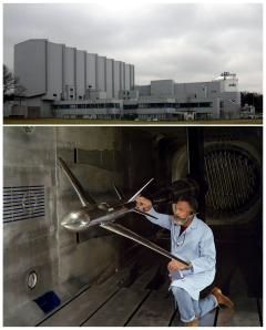
Figure 6.20:Buildings of the etw (European Transonic Windtunnel) in Cologne and test section of the National Transonic Facility of NASA, of similar size and capabilities.

Exercise 6.8

Electricity Generation With a Gas Turbine A gas turbine (in English the term gas turbine can be used to describe the engine as a whole) is set up to operate an electric generator (figure 6.21); it operates with a flow rate of $0.5 kg s^{-1}$ of atmospheric air. uration named turboshaft, powering an electric generator. The gas is typically expanded (in the turbine, between C and D) to atmospheric pressure. Diagram CC-by-sa Olivier Cleynen • The air enters the machine at $20^{\circ}C (68 ^{\circ} F)$ and 1 bar; it is compressed (A $\rightarrow$ B) to 30 bar in the compressor. • The air then receives heat through combustion, at constant pressure (B $\rightarrow$ C), until its temperature reaches $1000^{\circ}C$ . • Finally, the air is expanded in a turbine (C $\rightarrow$ D) until it reaches atmospheric pressure and is discharged outside. The compressor is mechanically powered by the turbine, and the shaft connecting them also drives the electric current generator. In order to quantify the maximum efficiency that could be achieved by the machine, we consider that the compressor and the turbine are reversible adiabatic (meaning that compression and expansion occur very slowly and without heat transfer). 1. Draw the process undergone by the air during one cycle on a pressure-volume diagram, qualitatively (that is, without showing numerical values). 2. At what temperature does the air exit the compressor? 3. What is the power of the compressor? 4. At what temperature is the air rejected into the atmosphere? What power is rejected as heat into the atmosphere? 5. What is the efficiency of the machine? 6. How do the four energy transfers of this theoretical machine compare to those of a real machine, where the compressor and the turbine cannot be reversible?

Answer

With equation 4/37, $T_{\mathrm{B}}= T_{\mathrm{A}}(\frac{p_{\mathrm{B}}}{p_{\mathrm{B}}} )^{\frac{\gamma -1}{\gamma}} = 774.7 K$ ;
With equations 3/14 and 4/14, $\dot{W}_{\mathrm{A}\rightarrow \mathrm{B}}=\dot{} mc_{p}(T_{\mathrm{B}}- T_{\mathrm{A}}) = +242 kW$ ;
With equation 4/37, $T_{\mathrm{D}}= T_{\mathrm{C}}(\frac{p_{\mathrm{D}}}{p_{\mathrm{C}}} )^{\frac{\gamma -1}{\gamma}} = T_{\mathrm{C}}(\frac{p_{\mathrm{B}}}{p_{\mathrm{A}}} )^{-\frac{\gamma -1}{\gamma}} = 481.8 K$ . Therefore, the rejected air must lose $\dot{Q}_{\mathrm{D}\rightarrow \mathrm{A}}= c_{p}\Delta T = -94.8 kW$ in order to return to its initial state (§6.2.1); honorable, only attainable with perfect turbine and compressor);
With a real compressor $\dot{W}_{\mathrm{A}\rightarrow \mathrm{B}_{2}}>\dot{W}_{\mathrm{A}\rightarrow \mathrm{B}}$ and $T_{\mathrm{B}_{2}}> T_{\mathrm{B}}$ . It follows that if $T_{\mathrm{C}}$ is kept constant, $\dot{Q}_{\mathrm{B}\rightarrow \mathrm{C}_{2}}<\dot{Q}_{\mathrm{B}\rightarrow \mathrm{C}}$ . Nevertheless, we still have $W_{\mathrm{C}\rightarrow \mathrm{D}_{2}}<\dot{W}_{\mathrm{C}\rightarrow \mathrm{D}}$ and $T_{\mathrm{D}_{2}}> T_{\mathrm{D}}$ in the turbine. The power $\dot{W}_{\mathrm{net}}$ decreases, the rejection $\dot{Q}_{\mathrm{out}}$ increases. We will see in chapter 7 (the second law) that the efficiency also decreases. Note: We had already studied this engine in problems 1.9 p. 29 and especially 3.2 p. 75. Our ability to analyze and quantify performance improves each time...

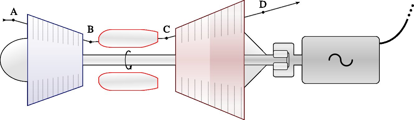
A static gas turbine engine, in this configuration named turboshaft, powering an electric generator. The gas is typically expanded (in the t — Figure 6.21:A static gas turbine engine, in this configuration named *turboshaft*, powering an electric generator. The gas is typically expanded (in the turbine, between C and D) to atmospheric pressure.

Exercise 6.9

Cycle of a Steam Engine In a steam power plant, water circulates continuously through four components: • A quasi-adiabatic pump where water enters as saturated liquid and its pressure is raised from 0.5 bar to 40 bar; • A boiler where its temperature is raised to $650^{\circ}C$ at constant pressure; • A quasi-adiabatic turbine that allows the water to return to 0.5 bar while expending energy as work; • A condenser that cools the water at constant pressure $(0.5 bar)$ until its return to the pump. We accept the following assumptions: • At the turbine outlet, the steam is at a temperature of $110^{\circ}C$ (after chapter 8, we will be able to predict this outlet temperature); • The compression in the pump is reversible, and the density of water does not vary as it passes through it. 1. Draw the process undergone by the water on a pressure-volume diagram, qualitatively (that is, without showing numerical values) and showing the saturation curve. 2. What is the efficiency of the engine? 3. What would happen if, in order to eliminate heat rejection, we removed the condenser by connecting the pump inlet directly to the turbine outlet?

Answer

To assist in constructing these diagrams, one can review figures 5.7 p. 121 and 5.9 p. 122, as well as section §5.4 p. 131.
$h_{\mathrm{A}}= h_{L\,0.5\,\mathrm{bar}}$ ; $h_{\mathrm{B}}= h_{\mathrm{A}}+ \int _{\mathrm{A}}^{\mathrm{B}}v\,\mathrm{d}p = h_{\mathrm{A}}+ v_{L}\Delta p$ (5/13 & 5/14 with $q_{\mathrm{A}\rightarrow \mathrm{B}}= 0$ ); $h_{\mathrm{C}}= h_{650^{\circ}\mathrm{C}\,\&\,4\,\mathrm{MPa}}$ ; $h_{\mathrm{D}}= h_{110^{\circ}\mathrm{C}\,\&\,0.05\,\mathrm{MPa}}$ . With these data, we easily calculate $\eta_{\mathrm{engine}}\equiv \left|\frac{w_{\mathrm{net}}}{q_{\mathrm{in}}}\right|= -\frac{w_{\mathrm{net}}}{q_{\mathrm{in}}}= -\frac{w_{\mathrm{turbine}}+w_{\mathrm{pump}}}{q_{\mathrm{boiler}}}= \frac{-(h_{\mathrm{D}}-h_{\mathrm{C}})+(h_{\mathrm{B}}-h_{\mathrm{A}})}{h_{\mathrm{C}}-h_{\mathrm{B}}}= 31.47\%$ (interesting insofar as any type of fuel can be used).
In this case, the pump would (almost) force the vapor to follow the path from D to C, bringing it back to a temperature of $650^{\circ}C$ and making it impossible to add heat in the boiler. We would then effectively have a machine made up of a turbine and a pump exchanging water: it would be impossible to generate work this way...

Exercise 6.10

Industrial Refrigeration A supermarket chain is seeking your expertise to assess the profitability of an ambitious project to renew a fleet of refrigerators. All supermarkets in the company use the same model of refrigerator. Its efficiency is $100 \%$ . You travel to a representative supermarket, which allows you to take measurements and quantify the thermal transfers of the building. You highlight that: • The power absorbed as heat by the cold chambers of the refrigerators, averaged over the year, is $80 kW$ . • In the winter, the building loses heat with an average power of $400 kW$ . It is heated with a heat pump unit of cop 4. • In the summer, the building absorbs heat with an average power of $160 kW$ . It is cooled with an air conditioning unit of cop 0.9. • During autumn and spring, the heating/cooling needs are almost negligible. The company is considering replacing its entire fleet of refrigerators with a model of $220 \%$ efficiency, which requires a significant investment. It has a total of 100 supermarkets and pays 0.15 AC per $kW h$ on average for electricity. What would be the annual financial savings generated by changing the refrigerator model?

Answer

In a supermarket, both in spring and autumn, the energy savings provided by the new refrigerators amount to $43.6 kW$ . In summer, the heat to be absorbed by the air conditioners is reduced. Therefore, an additional saving of $48.5 kW$ in electricity can be added at the level of the air conditioners. In winter, the heat required by the heat pumps is increased. Therefore, an additional expense of $10.9 kW$ must be added at the level of the heat pumps. In the end, this represents an annual savings of $1.672 \times 10^{12}J$ , or $69.7 k$ AC per supermarket, which must be compared to the required investment and the costs incurred (including the call for your expertise...).

Exercise 6.11

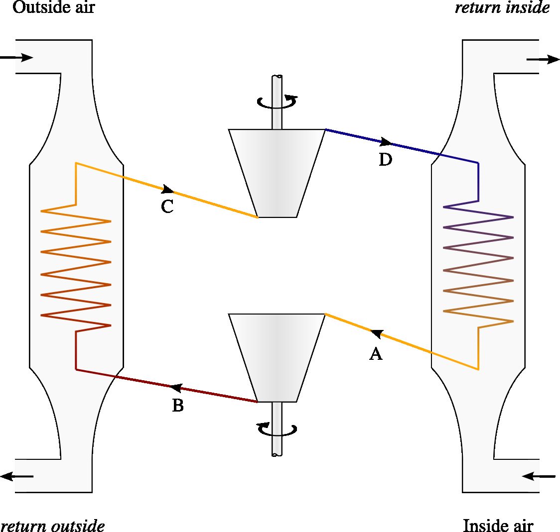
Operation of an AC Unit An air conditioner operates according to the circuit schematized in figure 6.22. The fluid used in the circuit is air (in practice, fluids that liquefy and evaporate within the machine are often used instead, but the operating principle remains the same). The air inside the circuit circulates in a steady flow. Both the compressor and the turbine are adiabatic and we consider them to be reversible. Heat transfers occur at constant pressure. When the air conditioner is started, the outside temperature and the inside temperature are both $86 ^{\circ} F (30^{\circ}C)$ . The temperatures of the air inside the circuit are $T_{\mathrm{A}}= 68 ^{\circ} F = 20^{\circ}C, T_{\mathrm{B}}= 140 ^{\circ} F = 60^{\circ}C$ , and $T_{\mathrm{C}}= 104 ^{\circ} F = 40^{\circ}C$ . 1. Draw the process qualitatively (that is, without showing numerical values) on a pressure-volume diagram; and indicate the work and heat transfers. 2. What is the pressure ratio between A and B? 3. What is the temperature of the air at point D? 4. Calculate the specific powers for each of the four energy transfers, and thus calculate the efficiency of the air conditioner. 5. The owner wants to obtain a flow of cool air at $53.6 ^{\circ} F (12^{\circ}C)$ with a flow rate of $529.7 CFM (0.25 m^{3}s^{-1})$ . What electrical power must be supplied to the air conditioner for this purpose? The air in the air conditioner circuit circulates in a steady flow (A $\rightarrow$ B $\rightarrow$ C $\rightarrow$ D $\rightarrow$ A), without ever leaving the machine. Diagram CC-by-sa Olivier Cleynen 6. What will be the minimum flow rate of outside air to be circulated in the outdoor section of the air conditioner? 7. During the winter, the owner wants to modify the air conditioner to turn it into a heat pump. Describe (qualitatively) a modification of the circuit for this purpose, and draw the process undergone by the air in the circuit on a new pressure-volume diagram, indicating the energy transfers.

Answer

With equation 4/37, $\dfrac{p_{\mathrm{B}}}{p_{\mathrm{A}}} = \left(\dfrac{T_{\mathrm{B}}}{T_{\mathrm{A}}}\right)^{\frac{\gamma}{\gamma -1}} = 1.565$ ;
Idem, expansion C → D is reversible adiabatic, $T_{\mathrm{D}}= T_{\mathrm{C}}\left(\dfrac{p_{\mathrm{D}}}{p_{\mathrm{C}}}\right)^{\frac{\gamma -1}{\gamma}}= T_{\mathrm{C}}\left(\dfrac{p_{\mathrm{A}}}{p_{\mathrm{B}}}\right)^{\frac{\gamma -1}{\gamma}}= T_{\mathrm{C}}\dfrac{T_{\mathrm{A}}}{T_{\mathrm{B}}} = 275.6\,\mathrm{K}$ or $2.4^{\circ}\mathrm{C}$ or $36.3^{\circ}\mathrm{F}$ ;
With equations 3/15 and 4/14, $w_{\mathrm{in}}= +40.2\,\mathrm{kJ\,kg^{-1}}$ ; $q_{\mathrm{out}}= -20.1\,\mathrm{kJ\,kg^{-1}}$ ; $w_{\mathrm{out}}= +37.76\,\mathrm{kJ\,kg^{-1}}$ ; $q_{\mathrm{in}}= +17.6\,\mathrm{kJ\,kg^{-1}}$ . Thus with equation 6/6, $\eta_{\mathrm{conditioner}}= 7.213$ ;
We want to obtain in 2 (return inside) $\dot{m}_{\mathrm{internal\,air}}= \dfrac{\dot{V}_{2}}{v_{2}} = \dfrac{\dot{V}_{2}p_{2}}{RT_{2}} = 0.305\,\mathrm{kg\,s^{-1}}$ . We must therefore remove a power $\dot{Q}_{\mathrm{internal\,air}}= \dot{m}_{\mathrm{internal\,air}}c_{p}(T_{2}- T_{1}) = -5.51\,\mathrm{kW}$ (3/14 & 4/14) from the internal air. The air conditioning unit will therefore require $\dot{W}_{\mathrm{net}}= \dfrac{-\dot{Q}_{\mathrm{internal\,air}}}{\eta_{\mathrm{conditioner}}} = 765\,\mathrm{W}$ .
To minimize $\dot{m}_{\mathrm{external\,air}}$ , we need to maximize its outlet temperature $T_{4}$ . However, we necessarily have $T_{4}\le T_{\mathrm{B}}$ , otherwise the heat transfer would occur in the wrong direction. Thus, $\dot{m}_{\mathrm{external\,air\,min.}}= \dfrac{-\dot{Q}_{\mathrm{out\,air\,conditioner}}}{c_{p}(T_{4\mathrm{max.}}-T_{3})} = \dfrac{-\dot{Q}_{\mathrm{in}}-\dot{W}_{\mathrm{net}}}{c_{p}(T_{4\mathrm{max.}}-T_{3})} = 0.208\,\mathrm{kg\,s^{-1}}$ (theoretical minimum).
In principle, it is sufficient to reverse the positions of the compressor and the turbine. In practice, the temperature ranges will also need to be shifted to allow heat absorption in cold weather.

Schematic diagram of an air conditioner. The air in the air conditioner circuit circulates in a steady flow (A B C D A), without ever leavin — Figure 6.22:Schematic diagram of an air conditioner. The air in the air conditioner circuit circulates in a steady flow (A $\rightarrow$ B $\rightarrow$ C $\rightarrow$ D $\rightarrow$ A), without ever leaving the machine.

Exercise 6.12

Conditioning Pack of an Aircraft

A “conditioning pack” or simply “air pack” is a thermodynamic machine used in commercial aircraft to pressurize the fuselage and to maintain the temperature in the cockpit, cabin, and cargo holds at a comfortable level regardless of external conditions.

The packs (often called ecs or acm, for Environment Control System and Air Cycle Machine) are often placed around the wing box in the unpressurized area of aircraft (figure 6.27). An interesting feature of their operation is that it is the air from the thermodynamic circuit itself that is inserted into the cabin for the passengers.

Here we study the heating and air conditioning functions of a conditioning pack: for this purpose, we model its operation in a simplified manner.

The air intended for the cabin begins its journey at the inlet of the jet engines of the airplane (except when the airplane, on the ground, is connected to a source of conditioned or pressurized air). In the compressor of one of these engines, its pressure is multiplied by 5 during an approximately adiabatic and reversible process; then it is led to the pack.

As it enters the pack, this air passes through a heat exchanger where it loses heat (figure 6.24). This heat is extracted by a separate air flow, called ram: it is air from outside at atmospheric conditions, extracted and discharged under the fuselage. The cabin air and ram air circuits are at very different pressures and are never mixed.

After passing through the heat exchanger, the air can follow three distinct circuits in the conditioning pack before reaching the cabin:

Circuit A is used in cold weather when one wants to raise or maintain the cabin at a higher temperature than the outside temperature;
Circuit B is used in moderate weather when the cabin needs to be kept at a temperature close to the outside temperature;
Circuit C is used in hot weather when there is a high demand for cabin air cooling.

The pack automatically controls the flow of outside air (ram) and selects the circuit for the air intended for the cabin to follow, in order to bring its temperature to the value requested by the crew in the cockpit (figure 6.28).

Circuit A: heating in cold weather

In circuit A, the air intended for the cabin is simply expanded in a valve (figure 6.25) before being inserted into the cabin.

In the valve, the pressure drops sharply and the specific volume increases; however, no work or heat transfer occurs. This is a process known as a “Joule & Gay-Lussac expansion” (see §4.3.2 p. 90). The process is entirely irreversible.

When the airplane is on the ground in cold weather conditions $(-35^{\circ}C, 1 bar$ or $-31 ^{\circ} F$ and $14.5 psi)$ :

What is the maximum temperature of the air that the pack can supply to the cabin? (for this, we will fully close the outside air ram circuit).
Draw the process qualitatively on a pressure-volume diagram.
What is the minimum flow rate of outside air required to circulate in the ram circuit in order to bring $0.5 kg/s$ of conditioned air at $24^{\circ}C (75 ^{\circ} F)$ into the cabin?
Draw the process that the conditioned air would undergo on the pressure-volume diagram above.

Circuit B: cabin air conditioning in moderate weather

In practice, it is possible to lower the temperature of the air intended for the cabin with a much lower ram air flow. For this reason, when cooling needs are significant, the air intended for the cabin goes through circuit B. It is then expanded using a turbine to the cabin pressure $(1 bar)$ . We assume that the turbine is ideal (reversible adiabatic expansion).

When the external conditions are $20^{\circ}C, 1 bar (68 ^{\circ} F$ and $14.5 psi))$ :

At what temperature will the air enter the cabin if the ram circuit is closed?
How much energy will be extracted from the air by the turbine?
Draw the process undergone by the air on a pressure-volume diagram, qualitatively.
What is the minimum temperature to which the circuit can bring the air intended for the cabin?
How much energy will be extracted from the air by the turbine in that case?
Draw the process on the pressure-volume diagram above.

Circuit C: cabin air conditioning in hot weather

When the aircraft is on the ground in very hot weather conditions $(45^{\circ}C$ or $113 ^{\circ} F, 1 bar)$ , the air intended for the cabin goes through circuit C.

Upon passing through the heat exchanger, its temperature only drops to $217^{\circ}C (422.6 ^{\circ} F)$ .

It is then compressed in a compressor (reversible adiabatic process) to $20 bar (290.1 psi)$ .

It then passes again through a heat exchanger crossed by the ram air circuit.

Finally, it is expanded in a turbine (in practice, this is the turbine used in circuit B) down to atmospheric pressure, and then fed into the cabin. We model the expansion as a reversible adiabatic process.

Make a sketch of the path followed by the air through the conditioner and draw the process qualitatively on a pressure-volume diagram.
At what temperature should the air be brought to in the second heat exchanger, before expansion, to obtain an air flow at $5^{\circ}C (41 ^{\circ} F)$ in the cabin?
What is the work that the pack receives or supplies to operate in this case?

Conclusion

What is the cop of the heating system generated with circuit A in question 3?
What is the cop of the air conditioning performed with circuit C in question 12?

Answer

If the ram circuit is closed, then $T_{3\mathrm{A}}= T_{2\mathrm{A}}$ ; and since $T_{4\mathrm{A}}= T_{3\mathrm{A}}$ (§4.3.2) we obtain $T_{4\mathrm{A}}= T_{1\mathrm{A}}(\frac{p_{2\mathrm{B}}}{p_{1\mathrm{B}}} ) ^{\frac{\gamma -1}{\gamma}}= 377.19 K = 104.1^{\circ}C = 219.4 ^{\circ} F$ .
In the ram exchanger we have $\dot{Q}_{\mathrm{cabin} \mathrm{air}}= -\dot{Q}_{\mathrm{ram} \mathrm{air}}$ so $\dot{m}_{\mathrm{cabin} \mathrm{air}}q_{\mathrm{cabin} \mathrm{air}}= -\dot{m}_{\mathrm{ram} \mathrm{air}}q_{\mathrm{ram} \mathrm{air}}$ or $\dot{m}_{\mathrm{cabin} \mathrm{air}}c_{p}(T_{3\mathrm{A}}- T_{2\mathrm{A}}) = -\dot{m}_{\mathrm{ram} \mathrm{air}}c_{p}(T_{\mathrm{ram} \mathrm{outlet}}- T_{\mathrm{ram} \mathrm{inlet}})$ . Thus, $\dot{m}_{\mathrm{ram} \mathrm{air}}$ is minimized when $T_{\mathrm{ram} \mathrm{outlet}}$ is maximized; now we necessarily have $T_{\mathrm{ram} \mathrm{outlet}}\le T_{2\mathrm{C}}$ . Thus, $\dot{m}_{\mathrm{ram} \mathrm{air} \min.}= -\dot{m}_{\mathrm{cabin} \mathrm{air}}\frac{T_{3\mathrm{A}}-T_{2\mathrm{A}}}{T_{2\mathrm{C}}-T_{\mathrm{ram} \mathrm{inlet}}}= 0.29 kg s^{-1}$ (so about $200 L s^{-1}$ or $424 CFM$ at the inlet).
If the ram circuit is closed, then $T_{3\mathrm{B}}= T_{2\mathrm{B}}$ ; we have $T_{4\mathrm{B}}= T_{3\mathrm{B}}\left(\frac{p_{4\mathrm{B}}}{p_{3\mathrm{B}}}\right)^{\frac{\gamma -1}{\gamma}}= T_{2\mathrm{B}}\left(\frac{p_{1\mathrm{B}}}{p_{2\mathrm{B}}}\right)^{\frac{\gamma -1}{\gamma}}= T_{1\mathrm{B}}= 293.15\,\mathrm{K} = 20^{\circ}\mathrm{C} = 68^{\circ}\mathrm{F}$ .
$w_{\mathrm{turbine} \mathrm{B}}= c_{p}(T_{4\mathrm{B}}- T_{3\mathrm{B}}) = -w_{\mathrm{compression} \mathrm{B}}= -172 kJ kg^{-1}$
We obtain $T_{4\mathrm{Bmin}.}$ when $T_{3\mathrm{B}}= T_{3\mathrm{Bmin}.}= T_{\mathrm{external}}$ . Then $T_{4\mathrm{Bmin}.}= T_{3\mathrm{Bmin}.}\left(\frac{p_{4\mathrm{B}}}{p_{3\mathrm{B}}}\right)^{\frac{\gamma -1}{\gamma}}= 185.1\,\mathrm{K} = -88.1^{\circ}\mathrm{C} = -127^{\circ}\mathrm{F}$ (a purely theoretical result, of course);
It decreases: $w_{\mathrm{turbine} \mathrm{B}2}= c_{p}(T_{4\mathrm{Bmin}.}-T_{3\mathrm{Bmin}.}) = -108.6 kJ kg^{-1}$ .
$T_{5\mathrm{C}}= T_{6\mathrm{C}}(\frac{p_{5\mathrm{B}}}{p_{6\mathrm{B}}} )^{\frac{\gamma -1}{\gamma}} = 654.6 K = 381.5^{\circ}C = 718.7 ^{\circ} F$ .
We first calculate $T_{4\mathrm{C}}= T_{3\mathrm{C}}(\frac{p_{4\mathrm{C}}}{p_{3\mathrm{C}}} )^{\frac{\gamma -1}{\gamma}} = 728.4 K$ . In the pack, the work transfers are $w_{\mathrm{pack}}= w_{\mathrm{pack} \mathrm{compressor}}+ w_{\mathrm{pack} \mathrm{turbine}}= c_{p}(T_{4\mathrm{C}}- T_{3\mathrm{C}}) + c_{p}(T_{6\mathrm{C}}- T_{5\mathrm{C}}) = -138.9 kJ kg^{-1}$ ; Thus, the air supplies net work in the pack, which in this case has a net surplus of shaft power.
In order to calculate these cop, the cycles must be completed by returning the air from the cabin condition back to the inlet condition (§6.2.1). In question 3 we have $\eta _{\mathrm{heat} \mathrm{pump}}= \left|\frac{q_{\mathrm{out}}}{w_{\mathrm{in}}}\right| = -\frac{c_{p}(T_{4\mathrm{A}}-T_{1\mathrm{A}})}{c_{p}(T_{2\mathrm{A}}-T_{1\mathrm{A}})} = 0.424$ (a rare application where a cop less than $100 \%$ is acceptable).
In question 12 we have $\eta_{\mathrm{conditioner}}= \left|\frac{q_{\mathrm{in}}}{w_{\mathrm{in}}}\right|= \frac{c_{p}(T_{1\mathrm{C}}-T_{6\mathrm{C}})}{c_{p}(T_{2\mathrm{C}}-T_{1\mathrm{C}}+T_{4\mathrm{C}}-T_{3\mathrm{C}}+T_{6\mathrm{C}}-T_{5\mathrm{C}})} = 0.842$ . In practice, however, the net work done by the air in the pack is not recovered: it is dissipated through friction into the ram air. We thus have $w_{\mathrm{net}}= c_{p}(T_{2\mathrm{C}}- T_{1\mathrm{C}})$ and the cop is decreased.

A few final comments: 1) In reality, adiabatic processes are not reversible, which further reduces the efficiencies calculated here. 2) The low values of these efficiencies result from compromises made to reduce the size, complexity, and especially the weight of the onboard systems. In this application, the available power as work is high, pneumatic energy is widely available, and any excess in volume or weight has disproportionate consequences. 3) In more recent aircraft (referred to as more electric), such as the B787 and the A350, the packs are now powered by electricity rather than using the same air intended for the cabin.

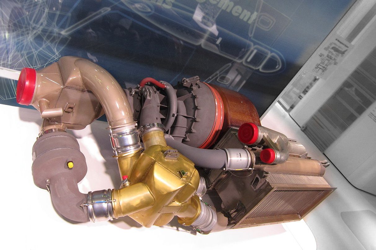
A ecs intended for a Comac C919, approximately in length. — Figure 6.23:A ecs intended for a Comac C919, approximately $1.5 m$ in length.

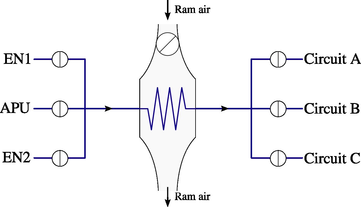
Figure 6.24:Diagram representing the air arriving in the conditioning pack from the engines (en1 and en2) or the auxiliary power unit (apu) on the left. This air exits into one of the three circuits A, B, or C after losing heat to the ram air.

Figure 6.25:Airflow regulation valve of an ecs intended for a Comac C919.

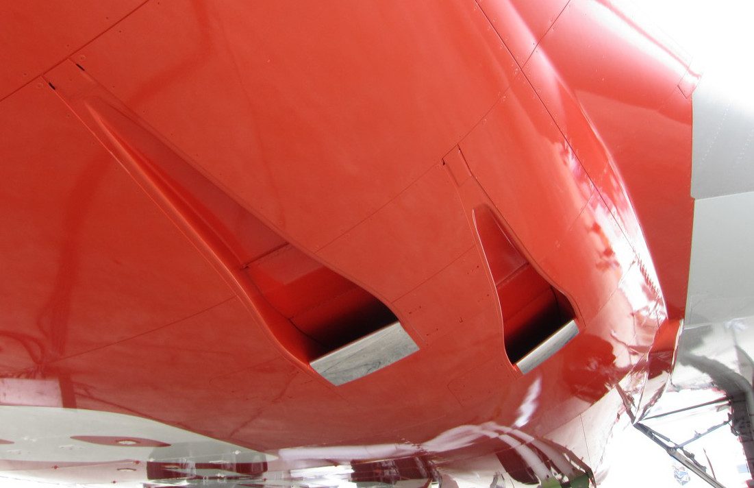
Figure 6.26:The air intakes of the ram circuit at the wing box of a Boeing 747-8I.

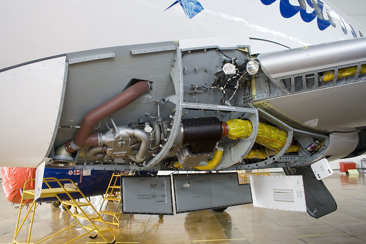
Figure 6.27:Air pack positioned at the wing root of a Sukhoi SuperJet SSJ100

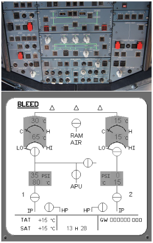
Figure 6.28:Control interface of the ecs in the center of the upper panel of the cockpit of an Airbus A320 and the corresponding efis display panel.

Photo CC-by-sa Olivier Cleynen

Footnotes¶

Some authors make a distinction between the efficiency $\eta$ defined in 6/3 and a relative efficiency or effectiveness $\Phi \equiv \frac{\eta _{\mathrm{real}}}{\eta _{\mathrm{theoretical}}}$ comparing the efficiency achieved in practice with the maximum achievable efficiency by the machine in theory. It is then necessary to carefully define the assumptions associated with the calculation of the maximum efficiency.
↩