5. Liquids and Vapors

Liquids and Vapors

The Dissociative Disorder of Liquefying Fluids

Introduction¶

This chapter 5 has exactly the same objectives as chapter 4 (the ideal gas), but applied to the study of fluids that liquefy and evaporate. It aims to answer two questions:

• How can we describe the behavior of a liquid or vapor they are heated or compressed?

• How can we predict the values of $u$ and $h$ when we use water in machines?

This chapter is incompatible with chapter 4 (the ideal gas) and we must forget everything that was learned there.

5.1 Evaporation and Condensation¶

5.1.1 What is a liquid?¶

A liquid is a fluid (namely, a substance without a definite shape) whose molecules are very close together, but still free to move relative to each other.

In concrete terms, a liquid is obtained from a gas by slowing down and bringing its molecules closer together. There is no chemical reaction involved. Thus, liquid water and water vapor are made of the same material (the same molecules): this material is just assembled differently.

Compared to gases, liquids have two important differences:

• They are practically incompressible, meaning that their specific volume $v$ varies very little when they are compressed;^[1]

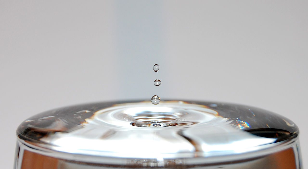
• They are subject to the effects of surface tension, which delights aesthetes and fluid mechanicists (figure 5.1), but is inconsequential in thermodynamics.

Figure 5.1:Surface tension gives liquids fascinating visual properties but has no consequence in thermodynamics. For us, it is the “same water” whether in the gaseous or liquid state.

5.1.2 Phase changes¶

Heating liquid water at ambient pressure (for example in a saucepan) makes it easy to see that the transition from the liquid state to the gaseous state occurs with a very large volume change. At 1 bar and $100^{\circ}C$ , the specific volume of water is multiplied by about a thousand before the temperature can increase again.

The abrupt change in one physical quantity while another changes is called a phase change. In this chapter, we will focus on the two phases: liquid and gaseous. In applications where it may change phase, we call a gas a vapor, and water vapor is called steam.

We will call the transition from liquid to vapor boiling or evaporation; conversely, the return from vapor to liquid is called condensation or liquefaction.

The concept of phase is difficult to define; there are many different phases (among which liquid, solid, gaseous, and plasma) and their boundaries are not always distinct. For example, we will see that it is possible to transform a liquid into vapor without ever observing boiling or abrupt property changes.

5.1.3 One way to approach evaporation and¶

condensation¶

When we explored the model of the ideal gas in §4.1.3, we had pictured molecules as very small billiard balls in chaotic motion, colliding with each other without ever being attracted one to the other (figure 4.1). In reality, molecules are also subject to respective attractive forces that greatly affect their behavior.

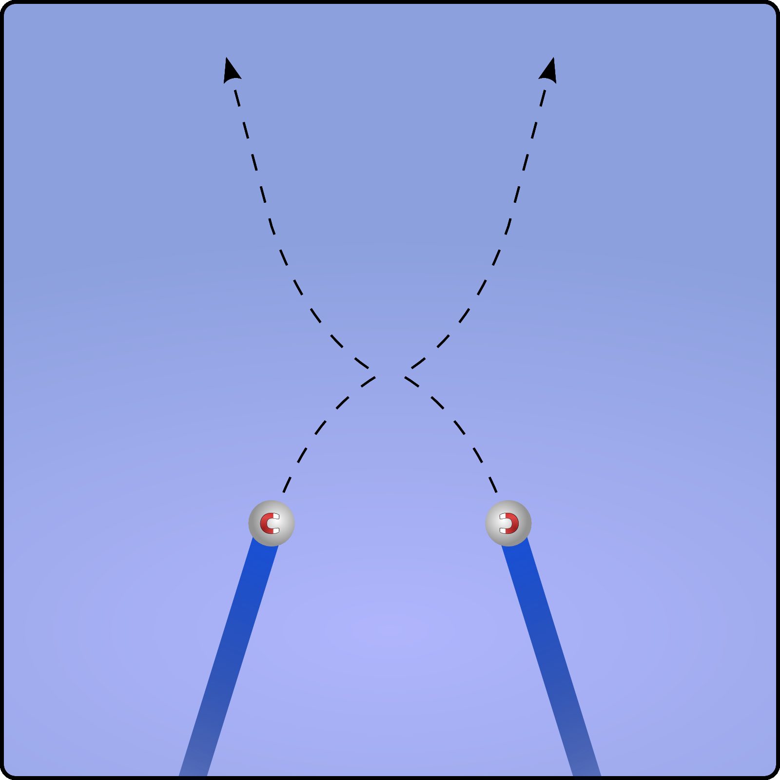
Let’s imagine, to start with, two very small billiard balls attracted to each other by a magnetic force and colliding without friction at very high speed (figure 5.2). The attracting force alters their trajectory when the balls are very close to each other; but once they move away, its influence becomes negligible.

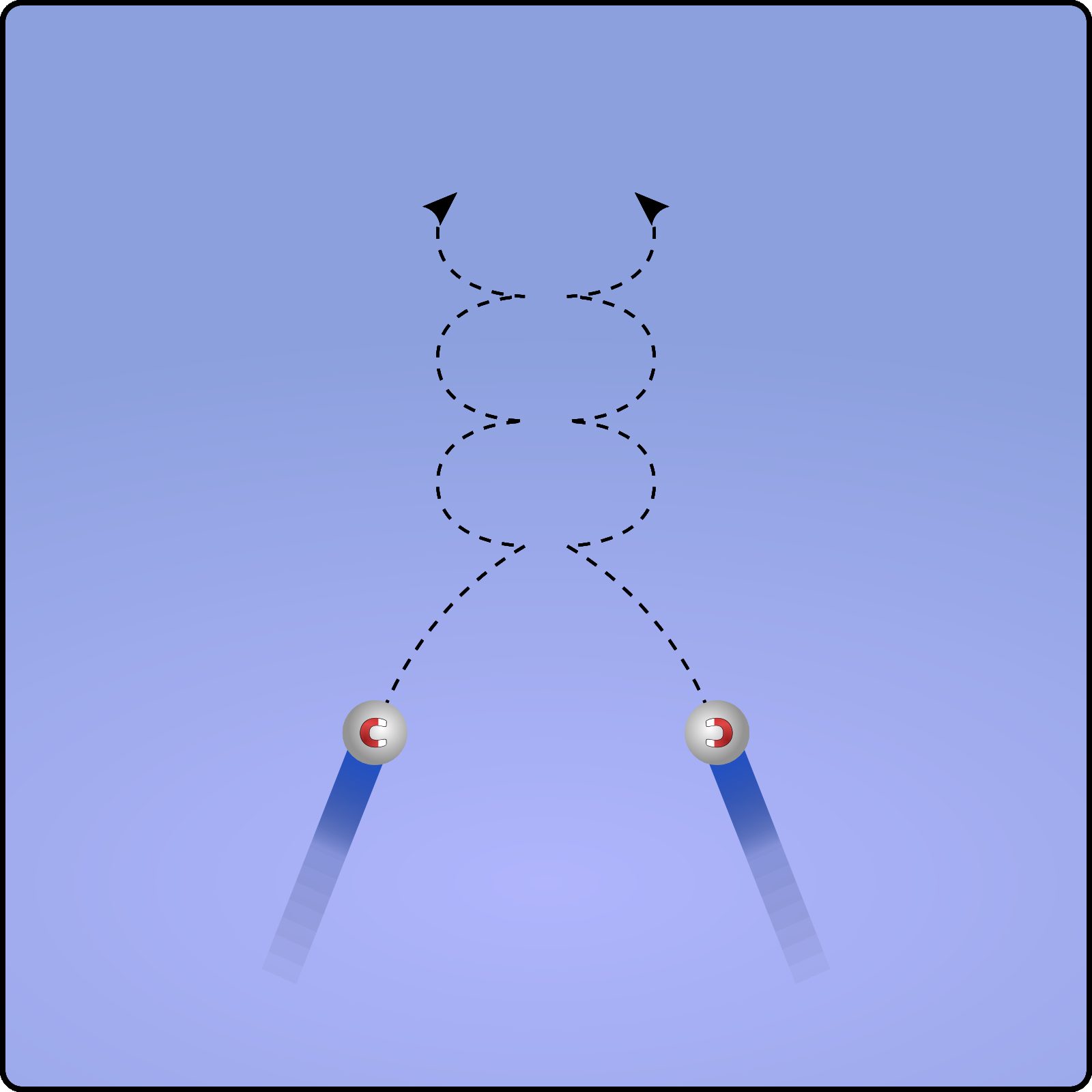
Now, let’s repeat the experiment with a lower initial speed (figure 5.3). There is a certain threshold speed below which the balls will not have enough kinetic energy to separate permanently. They will then form a pair, bouncing off each other periodically and occupying a significantly smaller average volume.

This simplistic model is a good initial approach to describe the phenomenon of condensation. When we reduce the kinetic energy of a vapor’s molecules (by cooling the vapor), once a critical threshold is crossed, they assemble much more compactly while continuing to collide at the same average speed (unchanged temperature). The more energy is extracted from the gas, the greater the number of molecules in compact interaction becomes. They form small groups; if they are numerous enough, the groups of 10¹⁴ (one hundred trillion) molecules scatter light and form a suspension that is visible to the naked eye. Droplets with a diameter of $0.1 mm$ contain

around 10^{16} molecules.

(1)

Any gas can thus be liquefied by cooling it and reducing its volume. The temperature and pressure required for liquefaction depend on the size and

Figure 5.2:Two magnetized billiard balls colliding without friction at high speed. The mutual attractive force alters the trajectory and behavior of the two balls, but only for a brief moment and over a short distance.

Diagram CC-by-sa by Commons User:Sharayanan & Olivier Cleynen

Figure 5.3:Two magnetized billiard balls colliding without friction at low speed. Below a threshold speed, the two balls will continue their trajectory together.

Diagram CC-by-sa by Commons User:Sharayanan & Olivier Cleynen geometry of the molecules that compose it. In the following sections, we will precisely quantify the amounts of energy and the ranges of properties required to vaporize and liquefy one fluid in particular: water.

5.1.4 Industrial use of water and liquids/vapors¶

When using a fluid to convert work and heat, it can be advantageous to exploit phase change phenomena.

In vapor form, a fluid behaves like a gas and spontaneously occupies all the volume made available to it. It is often used in this form to move mechanical parts (pistons in cylinders or blades in a turbine).

In liquid form, the fluid has a significantly higher density. It is often used in this form to transfer heat (heating or cooling) because much smaller conduits can be used. For example, in order to achieve the same power, a radiator filled with a gas should have a volume roughly a thousand times larger than if the fluid was liquefied.

Historically, water has been used in the very first engines in history for these reasons, and because changes in volume during phase changes allow for easier control of machines with low technology. Nowadays, liquids/vapors are mainly used in two major types of applications:

In power plants where liquids/vapors allow efficient heat extraction from external sources (waste combustion, nuclear reactions, geothermal energy). Water is used there, because it is abundant and easy to manipulate. Chapter 9 (steam power cycles) is entirely dedicated to these machines.

In refrigeration systems where liquids/vapors enable the use of compact components, especially pumps. The use of liquids/vapors also allows to drop the temperature of the fluid without having to use moving parts, using a simple valve, which is not possible with an ideal gas (see §4.3.2). A variety of fluids (then called “refrigerants,” although they are nothing extraordinary) are used for these purposes, selected according to their range of physical properties, cost, impact on the ozone layer, and contribution to global warming.

In this book, we focus on water, but the phenomena and calculation methods apply equally well to other liquids/vapors.

5.2 Qualitative Description of Water Properties¶

Properties¶

5.2.1 Limits of the ideal gas¶

As we slow down and bring the molecules of a gas closer together, the ideal gas model describes its properties less and less accurately. We observe a threshold below which liquefaction and evaporation occur, in other words, where the two liquid and gaseous phases coexist; this threshold is described in terms of a temperature and a pressure which are named critical. The critical temperatures and pressures of some common fluids are indicated in table 5.1. It should be noted that air, a mixture of several gases, will see different substances in its composition condense at different temperatures. When a fluid is maintained at a temperature and pressure significantly higher than its critical values, it behaves like an ideal gas. All fluids that we traditionally consider as liquids (for example, mercury) or gases (for example, CO $_{2})$ can transition from one state to the other.

Table 5.1:Critical temperatures and pressures of some substances. In practice, in the industry, engineers will mainly use the properties of two substances: water (in steam engines) and the refrigerant R-134a (in heat pumps and refrigerators). In this chapter, we will only use water, but the principles remain the same for all substances.

		$T_{\mathrm{cr}.}$ (K)	$p_{\mathrm{cr}.}$ (MPa)
Air	–	132	3.8
Chlorine	$\mathrm{Cl}_{2}$	417	7.71
Carbon dioxide	$\mathrm{CO}_{2}$	304.2	7.39
Water	$\mathrm{H}_{2}\mathrm{O}$	647.1	22.06
Helium	$\mathrm{He}$	5.3	0.23
Oxygen	$\mathrm{O}_{2}$	154.8	5.08
R-134a	$\mathrm{CF}_{3}\mathrm{CH}_{2}\mathrm{F}$	374.2	4.059
Xenon	$\mathrm{Xe}$	289.8	5.88

5.2.2 The temperature-volume $(T-v)$ diagram¶

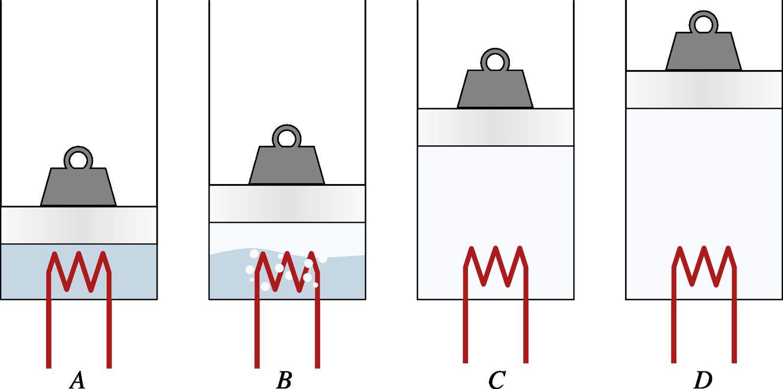
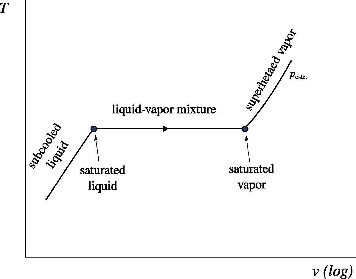
Let’s observe the temperature and volume of a mass of a liquid, here water, that is steadily heated while it is placed in a container at constant pressure (figure 5.4). Then we measure the temperature of the water as a function of its volume (figure 5.5).

Figure 5.4:Heating of a fixed quantity of water at constant pressure. A: subcooled liquid; B: liquid-vapor mixture; C: saturated vapor; D: superheated vapor.

Initially, when the water is liquid, the temperature increases linearly with the volume, with a steep gradient. This state is referred to as subcooled liquid (sometimes alternatively called compressed or unsaturated liquid).

Then, suddenly, while the volume continues to increase, the temperature stops rising. The mixture in the cylinder is now two-phase: part liquid, and part vapor. Adding heat does not cause any increase in temperature (unlike an ideal gas), but only the transformation of more liquid into vapor: this is called evaporation or boiling. In this state, the substance is called liquid-vapor mixture.^[2]

Figure 5.5:Vocabulary: states of the water during a process at constant pressure.

Diagram CC-0 Olivier Cleynen

Finally, once the last drop of liquid has been transformed into vapor, the temperature resumes its increase as more heat is added. The fluid is then in a state called dry or superheated vapor.

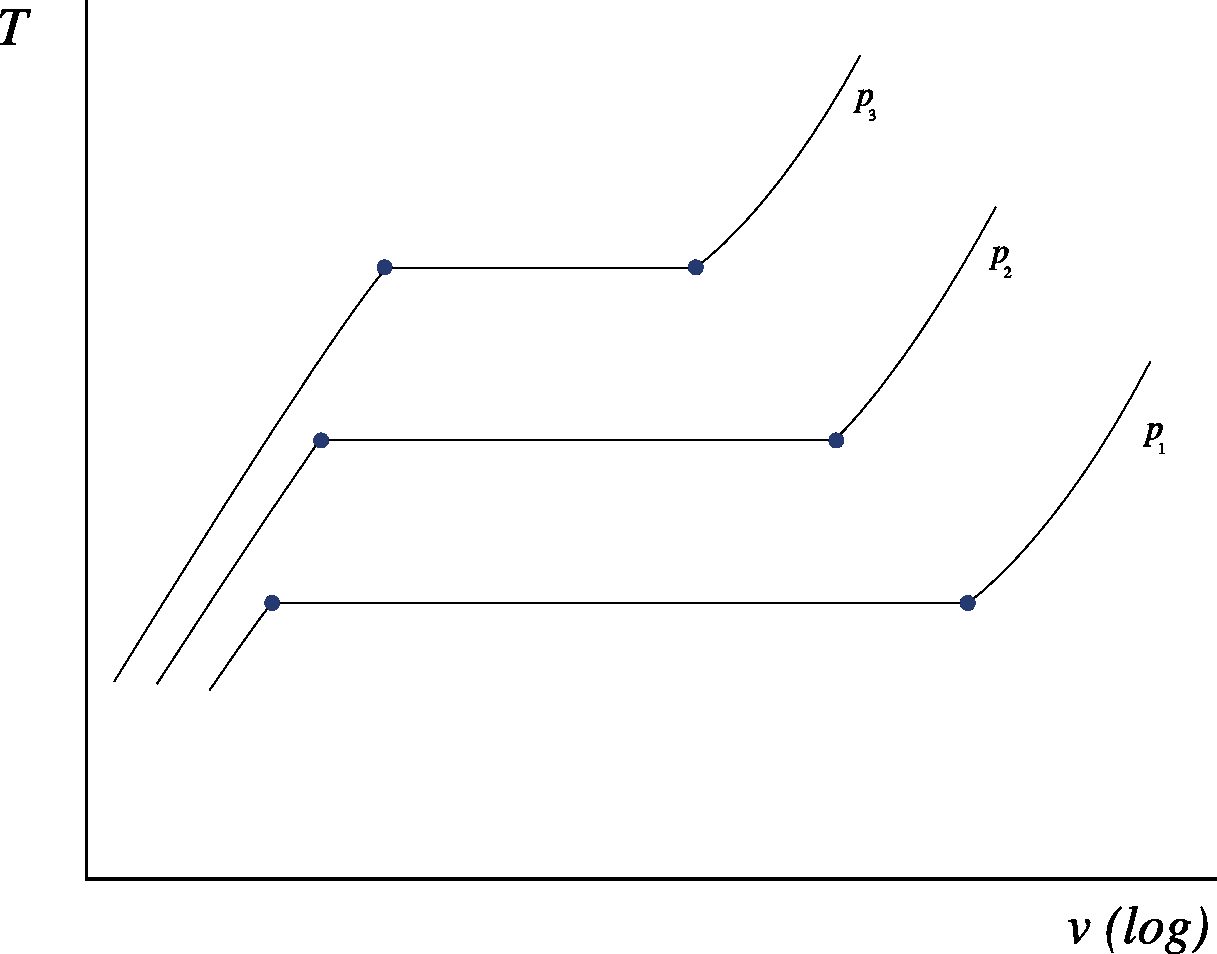
The experiment can be repeated at different pressures (figure 5.6). When the imposed pressure increases, two important facts are observed:

• The temperature of the phase change increases;

• The change of volume during the phase change is reduced.

Figure 5.6:Properties of water plotted on a temperature-volume diagram, when conducting the experiment described in figure 5.4 at different pressures. It can be observed that the higher the pressure, the smaller the boiling range becomes.

Diagram CC-0 Olivier Cleynen

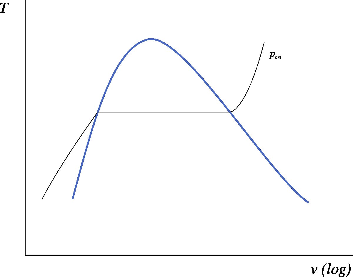
Above a certain pressure called critical pressure $p_{\mathrm{cr}.}$ , the phase change occurs indistinctly and there is no longer a range of constant temperature. The liquid turns into vapor without boiling!

At the end, we can connect all the phase change points, at all different pressures: we obtain a curve called saturation curve. All this information can be gathered on a temperature-volume $(T-v)$ diagram represented in figure 5.7, which well describes the properties of liquid-vapor mixtures. The student is encouraged to practice reproducing it.

Figure 5.7:Temperature-volume diagram of water, represented with a constant pressure (isobaric) process. The saturation curve is represented in blue.

Diagram CC-0 Olivier Cleynen

5.2.3 The pressure-volume diagram** $(p-v)$ ¶

In order to fully understand the phase change phenomenon, let’s now imagine a slightly different experiment.

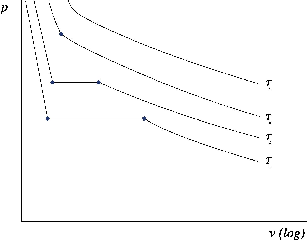
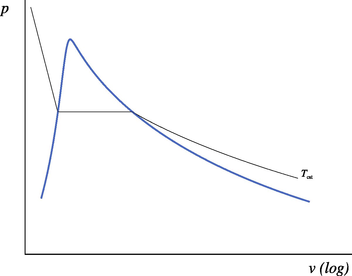
We propose to vary the volume of a given mass of fluid, again here water, while keeping its temperature constant (for example, by submerging the container in a lukewarm water bath). We then observe the pressure inside the container (figure 5.8).

As long as the water is liquid, we observe that the pressure drops sharply as we increase its volume. Then, suddenly, the pressure stops decreasing and remains perfectly constant, while the volume continues to increase: inside the cylinder, the water starts to boil and we have a liquid-vapor mixture. Finally, once the last drop of liquid water has evaporated in the cylinder, the pressure again starts to decrease.

If we replicate the experiment at different temperatures, we observe that the higher the temperature, and the shorter the phase change range becomes. Above a certain temperature, which we call critical temperature $(T_{\mathrm{cr}.})$ , the range disappears completely.

The behavior of a liquid-vapor in this experiment can be described on a pressure-volume $(p - v)$ diagram as shown in figure 5.9. The student is also encouraged to reconstruct this diagram.

Figure 5.8:Properties of water plotted on a pressure-volume diagram, when maintaining constant temperature by varying the volume.

Diagram CC-0 Olivier Cleynen

Figure 5.9:Pressure-volume diagram of water, represented with a constant temperature (isothermal) process. The saturation curve is represented in blue.

Diagram CC-0 Olivier Cleynen

5.2.4 A student’s false friend¶

The most important notion to remember from the behavior of liquid-vapors is that in contrast to ideal gases, their temperature is completely deregulated. It no longer simply dictates the other properties.

Let’s emphasize this. For a fluid close to a phase change:

pv \not\propto T

(5/1)

u \not\propto T

(5/2)

h \not\propto T

(5/3)

Almost everything that was covered in chapter 4 (the ideal gas) must be forgotten when dealing with a liquid/vapor. Fortunately, the first three chapters have not lost any of their utility.

5.2.5 Water in everyday life¶

The phenomena we describe here are easily observable and reproducible with water in everyday life. However, it should be noted that:

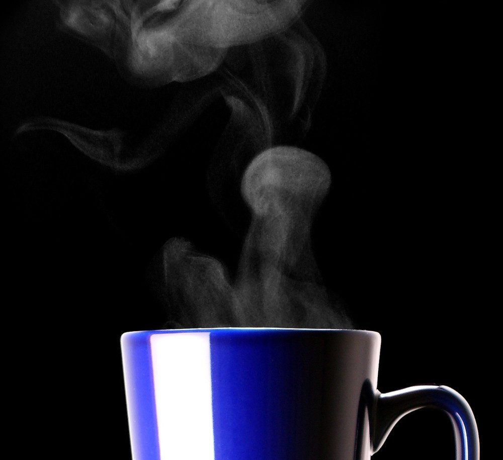
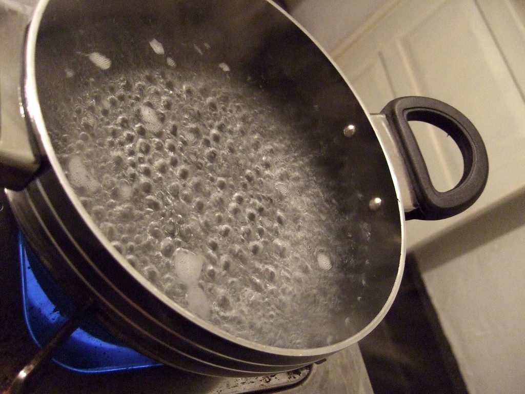
• Water vapor is transparent and almost invisible. What is observed above a boiling pot of water or in the form of clouds is liquid water suspended in the air (figure 5.10). These fine liquid droplets can gather to form drops (as a droplet grows, the surface area offering frictional resistance increases less rapidly than its weight, and its falling velocity increases) or evaporate again and become invisible once more.

Figure 5.10:The visible water above a container of hot liquid, sometimes called “steam”, is in the liquid state and not gaseous. These droplets are observable to the naked eye.

Photo by Jorge Barrios (public domain, cropped)

• Air is partially composed of water vapor (and its ability to carry water increases with temperature). When boiling liquid water in open air, it must not be forgotten that it is the air that hosts the water vapor; thus, the evaporation unfolds quite differently from the experiment described in figure 5.4. For example, the temperature of liquid water drops significantly during evaporation at constant pressure in the air. Another particularityis that condensation is catalyzed by the presence of dust particles in the air.

5.3 Quantifying the Properties of Water¶

For a liquid/vapor, there is no simple way to quantify the internal energy $u$ and enthalpy $h$ that interest us so much. Indeed, from $p$ and $v$ , we cannot calculate the temperature $(pv \not\propto T)$ and from $T$ , we cannot calculate $u$ and $h (u \not\propto T$ and $h \not\propto T)$ . • The bad news is that we will have to use tables of previously-measured properties, called steam tables, which can be tedious at times; • The good news is that these tables spare us from using the dreadful mathematical relations (such as $(T_{1}/T_{2})^{1/\gamma -1}= …)$ that described the properties of fluids in chapter 4 (the ideal gas).

5.3.1 Subcooled liquid and superheated vapor¶

Let’s start by heating a fixed amount of liquid water while maintaining its pressure constant, as we did in figure 5.4. For each temperature, we measure $v, u$ , and $h$ (as well as $s$ , but that’s a surprise we keep for chapter 8). The experiment is then repeated at a different pressure. The set of measurements is tabulated in Steam Table 1 (see pp. 306-309), of which an excerpt is presented in table 5.2.

Table 5.2:Excerpt from Steam Table 1 (see in Appendix A1 pp. 306-309). Here the measurements are made at $1.6 MPa$ , in other words, $16 bar (232 psi)$ . A discontinuity is observed between $200^{\circ}C$ and $300^{\circ}C$ : this is the state change that occurred at $T_{\mathrm{sat}.}= 201.37^{\circ}C$ , the saturation temperature for this

°C $T$	$m^{3}$ $kg$ $v$	$kJ$ $kJ$ $kg$ $kg$ $u$ $h$	$kJ$ $Kkg$ $s$
		$p = 1.6MPa$
		$(T_{\mathrm{sat}.}= 201.37^{\circ}C)$
10	0.001	42 43.6	0.1509
20	0.001001	83.8 85.4	0.2962
50	0.001011	209.1 210.7	0.7031
100	0.001043	418.6 420.3	1.306
200	0.001156	850.4 852.3	2.3305
300	0.15866	2781.5 3035.4	6.8863
500	0.22029	3120.1 3472.6	7.5409
600	0.24999	3293.9 3693.9	7.81
700	0.2794	3473.5 3920.5	8.0557
800	0.30865	3659.5 4153.3	8.2834
900	0.3378	3852.1 4392.6	8.4965
1000	0.36687	4051.2 4638.2	8.6974
1100	0.39589	4256.6 4890	8.8878
1200	0.42487	4467.9 5147.7	9.0689
1500	0.51169	5133.7 5952.4	9.5656
2000	0.65615	6326.8 7376.6	10.272

Here the measurements are made at $1.6 MPa$ , in other words, $16 bar (232 psi)$ .

A discontinuity is observed between $200^{\circ}C$ and $300^{\circ}C$ : this is the state change that occurred at $T_{\mathrm{sat}.}= 201.37^{\circ}C$ , the saturation temperature for this pressure.

This steam table allows us to answer many questions. Here are a few examples:

Example 5.2

How much energy does this water lose as it undergoes a process from $600^{\circ}C$ and 16 bar to $20^{\circ}C$ and 6 bar?

From Steam Table 1, at $1.6 MPa$ and $600^{\circ}C$ , we read $u_{1}= 3293.9 kJ kg^{-1}$ . For a pressure of $0.6 MPa$ at $20^{\circ}C$ , we read $u_{2}= 83.9 kJ kg^{-1}$ . We can then quantify the change in energy as $\Delta U = m(u_{2}- u_{1}) = -6420 kJ$ (hence a loss by the water).

We were able to quantify $\Delta U$ , but we cannot determine the proportions of heat $(Q_{1\rightarrow 2})$ and work $(W_{1\rightarrow 2})$ in this change. The less reversible the process, and the smaller the work $W_{1\rightarrow 2}$ will be compared to $Q_{1\rightarrow 2}$ . After chapter 8 (entropy), we will be able to use entropy to quantify the maximum amount of work that can be obtained between 1 and 2.

Example 5.3

A medium-sized turbine operates with a steam flow rate of $3 kg s^{-1} (6.61 lb/s)$ and a heat loss of $200 kW$ . At the inlet, the steam is at $600^{\circ}C$ and 16 bar; at the outlet, the steam is at 1 bar and $300^{\circ}C$ . What is the power delivered in the form of work?

At the inlet $(1.6 MPa$ and $600^{\circ}C)$ , we read $h_{1}= 3693.9 kJ kg^{-1}$ . At the outlet $(0.1 MPa$ and $300^{\circ}C)$ , we read $h_{2}= 3074.5 kJ kg^{-1}$ . Now, in an open system operating in steady state, neglecting changes in mechanical energy, we have $q_{1\rightarrow 2}+ w_{1\rightarrow 2}= \Delta h$ (equation 3/15). Therefore, $W_{1\rightarrow 2}=\dot{m} \Delta h-\dot{Q}_{1\rightarrow 2}= 3\times (3074.5\times 10^{3}-3693.9\times 10^{3})-(-200\times 10^{3}) = -1.6582 \times 10^{6}W = -1658.2 kW$ .

Example 5.4

What is the specific internal energy of water at 16 bar and $585^{\circ}C$ ?

We interpolate between two lines of Steam Table 1. We have $u_{500^{\circ}C}= 3120.1 kJ kg^{-1}$ and $u_{600^{\circ}C}= 3293.9 kJ kg^{-1}$ . We have progressed by a factor $y = \frac{585-500}{600-500} = 0.85$ between the two lines. We obtain by interpolation $u_{585^{\circ}C}= u_{500^{\circ}C}+ y \times (u_{600^{\circ}C}- u_{580^{\circ}C}) = 3267.83 kJ kg^{-1}$ .

After interpolating, always quickly check the order of magnitude of the results. Here $u_{585^{\circ}C}$ is indeed between $u_{500^{\circ}C}$ and $u_{600^{\circ}C}$ , and closer to $u_{600^{\circ}C}$ .

5.3.2 Saturation points¶

In order to precisely quantify the properties of water when it changes phase, we use Steam Tables 2 and 3. The properties of water in the form of saturated liquid (subscript $L)$ and saturated vapor (subscript $V)$ are tabulated for each temperature.

In Steam Table 2 (see pp. 310-311), the data is sorted by pressure (with each pressure corresponding to a single saturation temperature). Steam Table 3

(see pp. 312-313) presents exactly the same data, but sorted by temperature

(with each temperature corresponding to one saturation pressure). Excerpts from these steam tables are presented in Tables 5.3 and 5.4.

Table 5.3:Excerpt from Steam Table 2 (see in Appendix A1 pp. 310-311). Subscript $L$ corresponds to saturated liquid, and subscript $V$ corresponds to saturated vapor. The difference between these values is sometimes noted with an index $LV$ : for example $u_{LV}\equiv \Delta u_{L)V}\equiv u_{V}- u_{L}$ .

$T_{\mathrm{sat}.}$ (°C)	$p_{\mathrm{sat}.}$ (MPa)	$u_{L}$	$u_{V}$	$\Delta u_{L)V}$	$h_{L}$	$h_{V}$	$\Delta h_{L)V}$	$v_{L}$	$v_{V}$
⋮	⋮	⋮	⋮	⋮	⋮	⋮	⋮	⋮	⋮
115	0.16918	482.4	2523.4	2041	482.6	2698.6	2216	0.001056	1.0358
120	0.19867	503.6	2528.8	2025.2	503.8	2705.9	2202.1	0.00106	0.89121
125	0.23224	524.8	2534.3	2009.4	525.1	2713.1	2188	0.001065	0.77003
130	0.27028	546.1	2539.6	1993.5	546.4	2720.1	2173.7	0.00107	0.668
⋮	⋮	⋮	⋮	⋮	⋮	⋮	⋮	⋮	⋮

Table 5.4:Excerpt from Steam Table 3 (see in Appendix A1 pp. 312-313). These are the same data as in Steam Table 2; they are merely sorted by pressure instead of temperature.

$p_{\mathrm{sat}.}$ (MPa)	$T_{\mathrm{sat}.}$ (°C)	$u_{L}$	$u_{V}$	$\Delta u_{L)V}$	$h_{L}$	$h_{V}$	$\Delta h_{L)V}$	$v_{L}$	$v_{V}$
⋮	⋮	⋮	⋮	⋮	⋮	⋮	⋮	⋮	⋮
0.2	120.21	504.5	2529.1	2024.6	504.7	2706.2	2201.5	0.001061	0.88568
0.25	127.41	535.1	2536.8	2001.8	535.3	2716.5	2181.1	0.001067	0.71866
0.3	133.52	561.1	2543.2	1982.1	561.4	2724.9	2163.5	0.001073	0.60576
0.35	138.86	583.9	2548.5	1964.7	584.3	2732	2147.7	0.001079	0.52418
⋮	⋮	⋮	⋮	⋮	⋮	⋮	⋮	⋮	⋮

We can already answer simple questions using these tables:

Example 5.6

What is the increase in volume when water is vaporized at $130^{\circ}C$ ?

Water goes from a volume $v_{L}$ (a liquid just about to boil) to a volume $v_{V}$ (when the last drop has evaporated). We refer to Steam Table 2 (excerpt in table 5.3) where the data is sorted by temperature. At $130^{\circ}C$ , the specific volume increases by $v_{LV}\equiv \Delta v_{L)V}\equiv v_{V}- v_{L}= 0.668 - 0.001 07 = 0.666 93 m^{3}kg^{-1}$ (it is multiplied by about $600)$ .

Here, evaporation occurs entirely at $130^{\circ}C$ (which is quite easy to achieve in practice, since it simply involves maintaining constant pressure, see figure 5.7). If the temperature and pressure were not held constant, the final volume would be different.

Example 5.7

How much heat is needed to fully (and slowly) vaporize $4 L$ of saturated liquid water at 3 bar?

The water will receive heat, but will also do work (by expanding at constant pressure of $3 bar)$ . We will calculate $q_{\mathrm{evap}.}= q_{1\rightarrow 2}= (u_{2}- u_{1}) - w_{1\rightarrow 2}$ (equation 2/2). The water starts as a saturated liquid (state 1 = subscript $L)$ and ends up as a saturated vapor (state 2 = subscript $V)$ . Since the process is slow and at constant pressure, the work $w_{1\rightarrow 2}= -\int ^{2}_{1}pdv$ simply becomes $-p_{\mathrm{cst}.}(v_{2}- v_{1})$ . Let’s gather all of this information in one equation: $q_{\mathrm{evap}.}= (u_{V}-u_{L}) + p_{\mathrm{cst}.}(v_{V}- v_{L}) = h_{V}- h_{L}= h_{LV}\equiv \Delta h_{L)V}= 2163.5 kJ kg^{-1}$ . At 3 bar, our $4 L$ of saturated liquid water corresponds to a mass $m = \frac{V}{v_{L}} = \frac{4\times 10^{-3}}{0.001073} = 3.7279 kg$ . So, in the end, $Q_{\mathrm{evap}.}= m q_{\mathrm{evap}.}= 8065.2 kJ$ .

If we had used the usual approximation of 1000 liters per cubic meter of liquid water $(v_{L}\approx 10^{-3}m^{3}kg^{-1})$ , we would have made an error of +7.3%.

It is worth mentioning that the term $h_{LV}\equiv \Delta h_{L)V}\equiv h_{L}- h_{V}$ is sometimes called heat of vaporization or latent heat. Indeed, for evaporation in a closed system at a given temperature, $q_{\mathrm{evap}.}= \Delta u-w_{\mathrm{evap}.}= (u_{V}-u_{L}) + p_{\mathrm{sat}.}(v_{V}- v_{L}) = h_{LV}$ (the same result is obtained in an open system).

5.3.3 The liquid-vapor mixture¶

Finally, we want to quantify the properties of water between the saturation points, in other words, when it is only partially liquid. Experiment shows that in this region, fluids behave linearly, and its properties can be easily quantified.

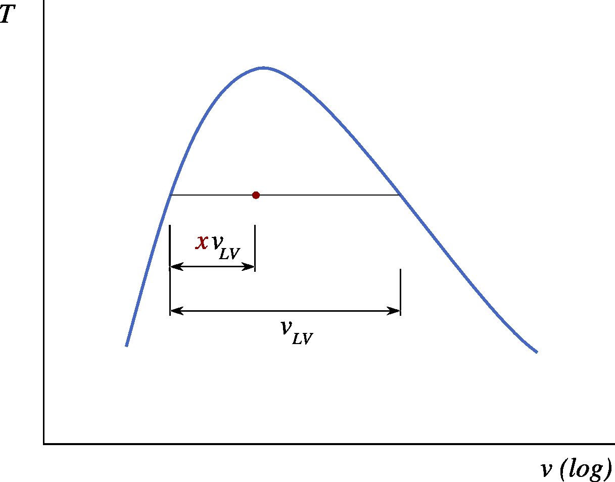
In order to “position” a liquid-vapor mixture between the two saturation points, we define the quality or dryness fraction as follows:

For example, a mass of $1 kg$ of water with a dryness fraction of 0.2 contains $0.8 kg$ of saturated liquid and $0.2 kg$ of saturated vapor. This $0.2 kg$ does occupy the majority of the available volume. We could say that the dryness fraction quantifies the progression of a liquid-vapor mixture between its two saturation points (figure 5.11). The concept of dryness fraction applies only to two-phase mixtures, thus we always have $0 \le x \le 1$ .

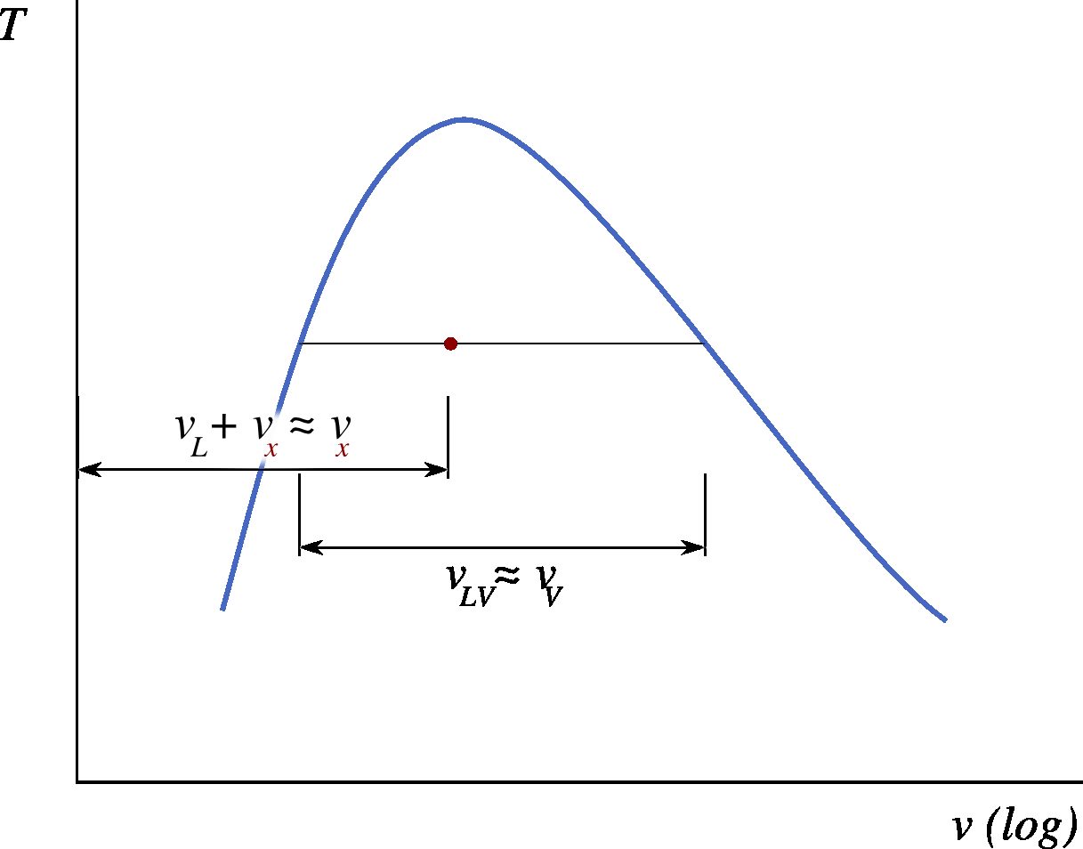
The vapor dryness fraction represented by the point position on a diagram. — Figure 5.11:The vapor dryness fraction represented by the point position on a $T -v$ diagram.

Diagram CC-0 Olivier Cleynen

We can now express the properties $u, h$ , and $v$ in terms of the dryness fraction:

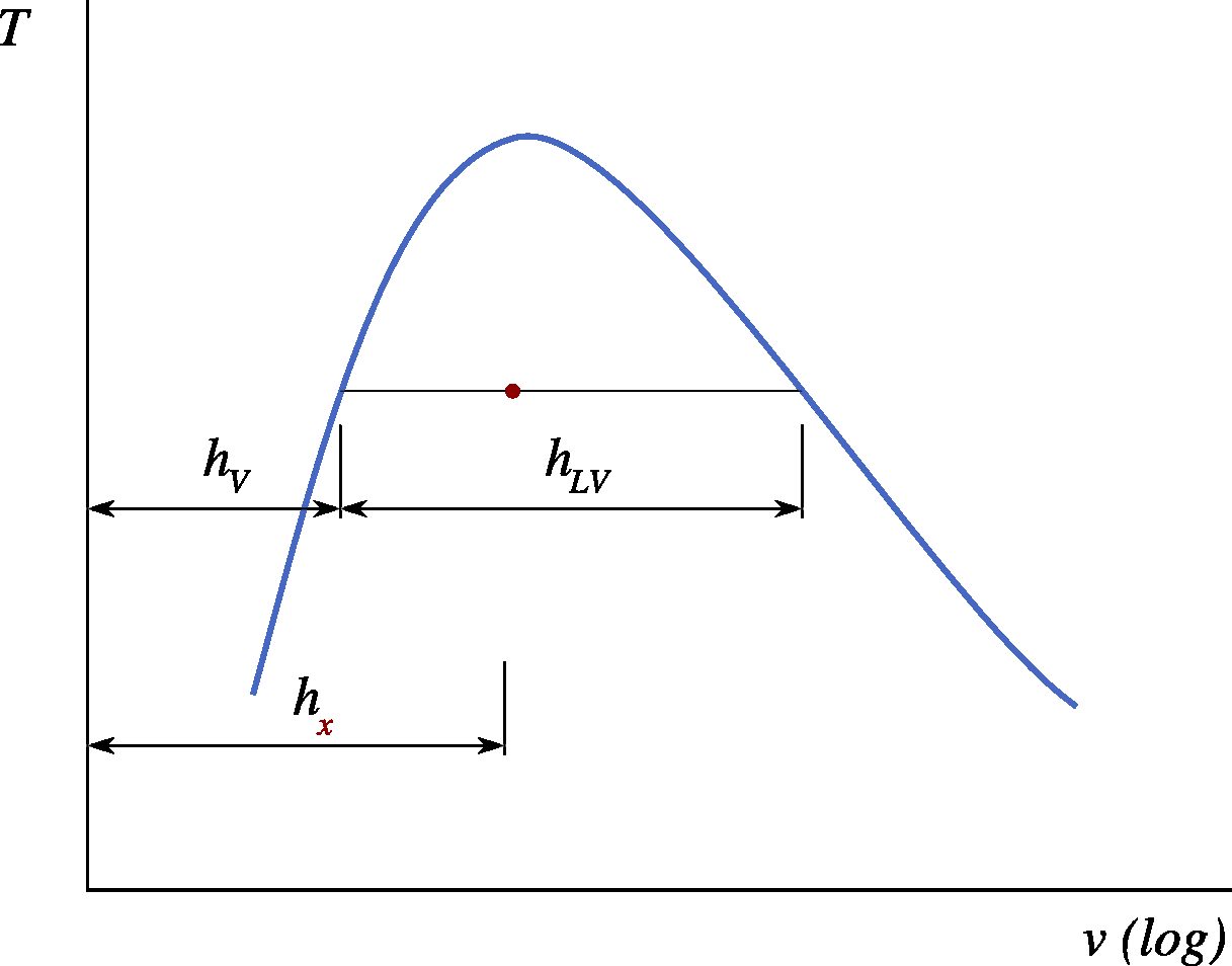
The enthalpy $h$ of a liquid-vapor mixture is equal to the sum of the enthalpy of the liquid and that of the vapor. We have, as illustrated in figure 5.12:

h_{x}= (1 - x)h_{L}+ x h_{V}

(2)

= h_{L}+ x(h_{V}- h_{L})

(3)

h_{x}= h_{L}+ x h_{LV}

(5/4)

where $h_{x}$ is the specific enthalpy of the mixture at hand $(J kg^{-1})$ , $x$ is its dryness fraction (unitless), and $h_{LV}\equiv \Delta h_{L)V}\equiv h_{V}- h_{L}$ (tabulated value) is the specific enthalpy of vaporization at its temperature $(J kg^{-1})$ .

Enthalpy of a mixture as a function of the enthalpies in the saturated state and of vaporization. — Figure 5.12:Enthalpy $h_{x}$ of a mixture as a function of the enthalpies in the saturated state and of vaporization.

Diagram CC-0 Olivier Cleynen

The internal energy $u$ of a liquid-vapor mixture is quantified in exactly the same way:

u_{x}= u_{L}+ x u_{LV}

(5/5)

where $u_{x}$ is the specific energy of the mixture under study $(J kg^{-1})$ , $x$ is its dryness fraction (unitless), and $u_{LV}\equiv \Delta u_{L)V}\equiv u_{V}-u_{L}$ (tabulated value) is the difference of specific internal energies at saturation, at its temperature $(J kg^{-1})$ .

The specific volume of a liquid-vapor mixture, finally, is quantified even more simply. The total volume of the mixture equals the volume of the gas plus the volume of the liquid, thus:

v_{x}= (1 - x)v_{L}+ x v_{V}

(4)

However, the specific volume $v_{L}$ of the saturated liquid is usually small compared to that of the vapor. A brief examination of Steam Table 2 will reveal that this is approximately a factor of 10³ (this factor is not very well highlighted by the $T - v$ and $p - v$ diagrams in this chapter, whose abscissa scales are logarithmic). We can therefore neglect $v_{L}$ and simply write:

v_{x}\approx x v_{V}

(5/6)

where $v_{x}$ is the specific volume of the mixture under study $(m^{3}kg^{-1})$ , $x$ is its dryness fraction (unitless), and $v_{V}$ (tabulated value) is the specific volume of the saturated vapor at its temperature $(m^{3}kg^{-1})$ .

This approximation is illustrated in figure 5.13.

We can now use the same Steam Tables 2 and 3 to quantify what happens between the saturation points.

Approximations used in calculating the volume occupied by a liquid-vapor mixture. It should be noted that the abscissa scale is logarithmic: $v_{L}$ is generally several hundred times smaller than $v_{V}$, and the approximation is not graphically emphasized. — Figure 5.13:Approximations used in calculating the volume occupied by a liquid-vapor mixture. It should be noted that the abscissa scale is logarithmic: $v_{L}$ is generally several hundred times smaller than $v_{V}$ , and the approximation is not graphically emphasized.

Diagram CC-0 Olivier Cleynen

Example 5.8

What is the internal energy and volume occupied by a mass of $4 kg$ of water, $75 \%$ vaporized, at $115^{\circ}C (239 ^{\circ} F)$ ?

We have a liquid-vapor mixture and the dryness is 0.75. We refer to Steam Table 2 (excerpt in table 5.3) to find the saturation temperature of $115^{\circ}C$ . Then, we simply apply equation 5/5: $u_{x}= u_{L}+ 0.75 \times u_{LV}= 482.4 + 0.75 \times 2041 = 2013.15 kJ kg^{-1}$ . Similarly, with equation 5/6: $v_{x}= 0.75 \times v_{V}= 0.75 \times 1.0358 = 0.776 85 m^{3}kg^{-1}$ . Therefore, we have $U = m u = 8052.6 kJ$ and $V = m v = 3.1074 m^{3}= 820.89 US gal$ .

5.4 Elementary Reversible Processes¶

We are now able to quantify the terms $pv, u$ , and $h$ of a liquid/vapor in all cases. Here, we intend to proceed just as in the previous chapter (§4.4): we want to calculate the energy transfers involved when compressing or expanding a liquid/vapor under entirely arbitrary constraints of volume, pressure, or temperature.

5.4.1 What is this chapter section for?¶

The answer is the same as in chapter chapter 4 (the ideal gas) (§4.4.1). The liquid/vapor processes we study here are highly hypothetical but interesting for two reasons:

The behavior of a liquid/vapor is intrinsically complex. These elementary processes serve as exercises to learn how to describe it step by step;
These elementary processes are conceptual tools that we will later assemble: first to quantify the theoretical limits of machines (in chapter 7), and finally to describe the behavior of fluids in industrial machines (in chapter 9).

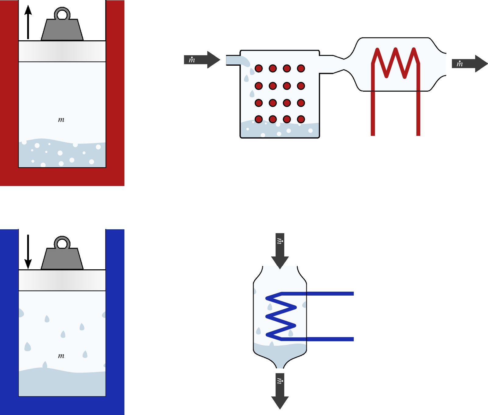
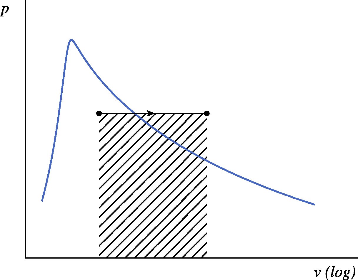
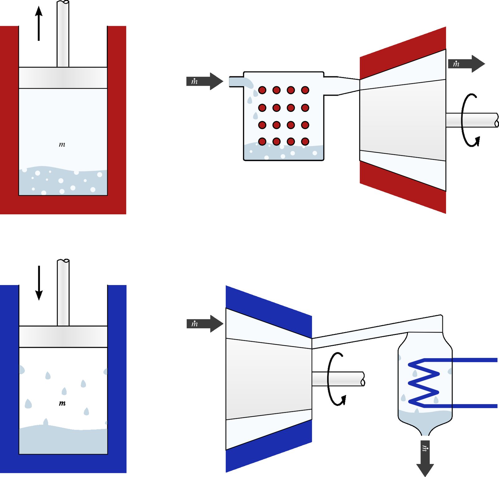
5.4.2 Processes at constant pressure¶

It is possible to heat or cool a liquid/vapor while maintaining its pressure constant (figure 5.14). A process at constant pressure is called isobaric. To generate one, we should:

• with a fixed amount of fluid (closed system), constrain it with a surface that exerts a constant force regardless of the volume;

• with fluid in steady flow (open system), simply transfer heat by letting it flow through a conduit without moving parts. This is what happens in a boiler or condenser, for example.

In a closed system, we have $q_{1\rightarrow 2}+ w_{1\rightarrow 2}= \Delta u$ (2/2). If the process is reversible, both heat and work can be quantified as follows:

w_{1\rightarrow 2}= -\int_{1}^{2} pdv = -p_{\mathrm{cst}.}\int_{1}^{2} dv

(5)

w_{1\rightarrow 2}= -p_{\mathrm{cst}.}\Delta v

(5/7)

in a reversible process at constant pressure $p_{\mathrm{cst}.}$ , in a closed system.

q_{1\rightarrow 2}= \Delta u - w_{1\rightarrow 2}= \Delta u + p_{\mathrm{cst}.}\Delta v

(6)

q_{1\rightarrow 2}= \Delta h

(5/8)

in a reversible process at constant pressure, in a closed system.

In an open system, we have $q_{1\rightarrow 2}+ w_{1\rightarrow 2}= \Delta h$ (3/15). If the process is reversible, both heat and work can be quantified as follows:

w_{1\rightarrow 2}= \int_{1}^{2} vdp

(7)

w_{1\rightarrow 2}= 0

(5/9)

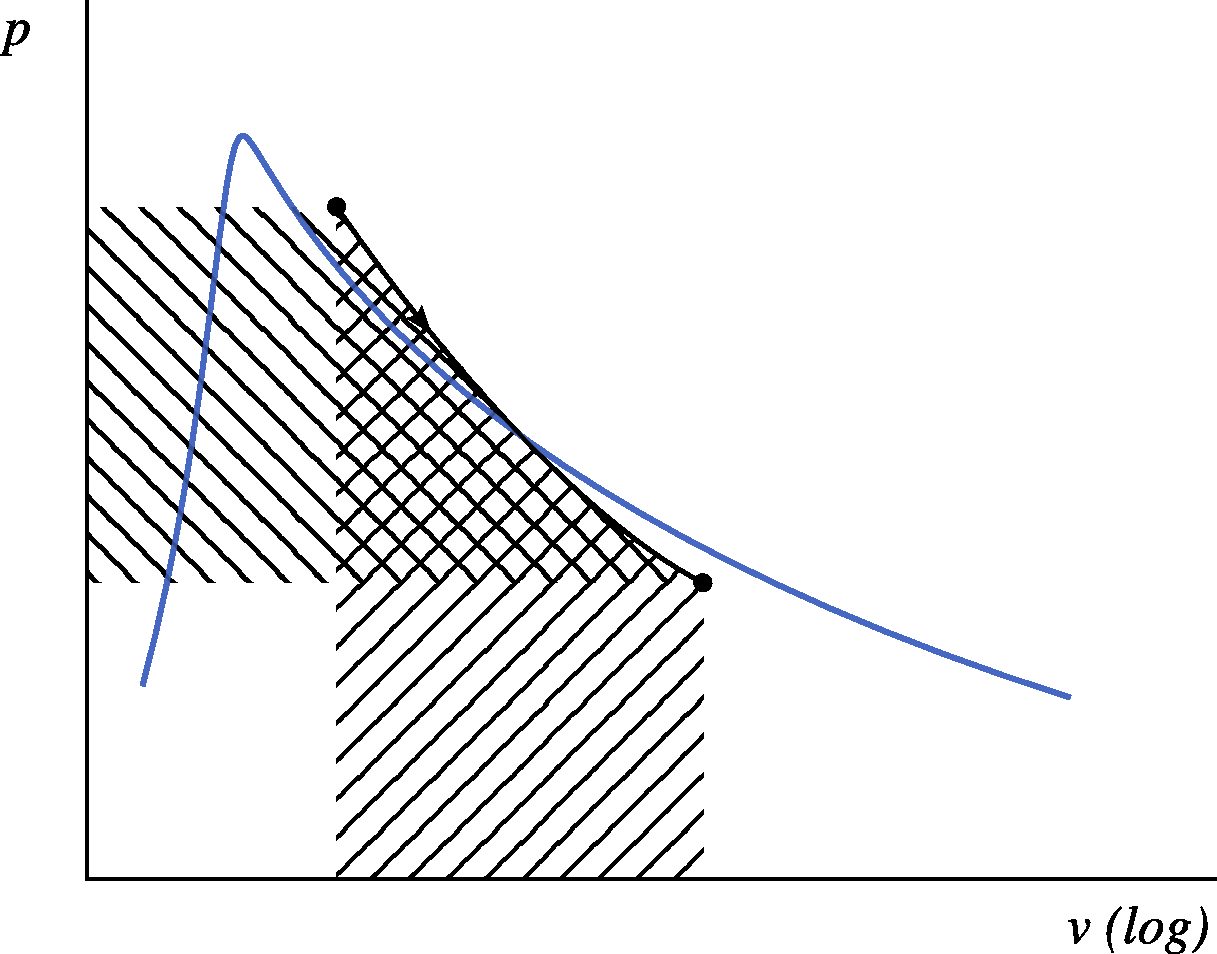
Figure 5.14:Constant-pressure (isobaric) process undergone by a liquid/vapor. In a closed system (on the left), the piston exerts a constant force throughout the process. In an open system (on the right), no work is done.

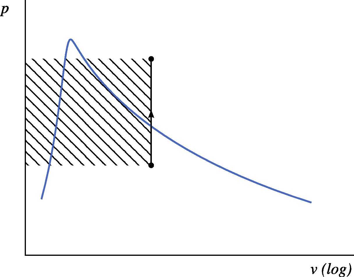
Diagram CC-by-sa Olivier Cleynen

Figure 5.15:Heating at constant pressure of a liquid/vapor, represented on a pressure-volume diagram.

Diagram CC-0 Olivier Cleynen

in a reversible process at constant pressure, in an open system.

q_{1\rightarrow 2}= \Delta h - w_{1\rightarrow 2}

(8)

q_{1\rightarrow 2}= \Delta h

(5/10)

in a reversible process at constant pressure, in an open system.

Example 5.10

How much work and heat are needed to slowly heat $2 kg$ of saturated liquid water at constant pressure $(3 bar)$ until the volume reaches $1 m^{3}$ ?

We start from the saturated liquid state, with $v_{1}= v_{L}$ and $h_{1}= h_{L}$ . We need the final specific volume and enthalpy in order to quantify $W_{1\rightarrow 2}$ and $Q_{1\rightarrow 2}$ . The final volume will be $v_{2}= \frac{V_{2}}{m} = 0.5 m^{3}kg^{-1}$ .

We notice that $v_{2}$ is less than $v_{V}$ at our temperature. At the end of the heating process, the water will still be partially liquid, and we will need to calculate its dryness fraction.

Liquid-vapor mixture? We are heading towards Steam Tables 2 and 3. We know the pressure $(0.3 MPa)$ , therefore we need Steam Table 3.

The final dryness fraction is $x_{2}\approx \frac{v_{x}}{v_{V}} = \frac{0.5}{0.60576} = 0.825$ (equation 5/6). Therefore, $h_{2}= h_{L}+ x_{2}h_{LV}= 561.4 + 0.825 \times 2163.5 = 2347.2 kJ kg^{-1}$ (5/4).

The work is obtained using equation 5/9: $W_{1\rightarrow 2}= m w_{1\rightarrow 2}= -mp_{\mathrm{cst}.}\Delta v = -2\times 0.3\times 10^{6}\times (0.5-0.001 073) = -2.994\times 10^{5}J = -299.4 kJ$ .

Finally, the heat transfer is calculated using equation 5/10: $Q_{1\rightarrow 2}= m q_{1\rightarrow 2}= m \Delta h = 2 \times (2347.2 \times 10^{3}- 561.4 \times 10^{3}) = +3.5715 \times 10^{6}J = +3571.5 kJ$ .

The heat transfer involved is ten times more significant than the work done. In this case, we are heating a lot, and the fluid, at low pressure, does little work.

It is probably simpler and less risky to derive these equations 5/9 and 5/10 by hand rather than trying to memorize them.

One can notice that when heating water in a liquid/vapor mixture (below the saturation curve), the volume increase is significant. In practice, just a few milliliters of liquid water can lead to an expansion of several liters at constant pressure, with a very moderate and constant temperature. This is why all the early engines, in the 19th century, operated with water rather than air. The large volume amplification allowed for more compact engines with large strokes (simpler mechanisms), the constant pressure meant forces were easier to manage, and the modest temperatures allowed the use of simple materials. This combination made the liquid-vapor mixture of water appealing at a time when metallic technology was limited. We will see in chapters 7 (the second law) and 9 (steam power cycles) that these advantages unfortunately translate into staggeringly low efficiencies. In order to overcome this, the temperature must be increased: that would be for the 20th century.

5.4.3 Processes at constant volume¶

It is possible to transfer heat to or from a liquid/vapor while maintaining its volume constant (figure 5.16). A process at constant volume is called an isochoric process. To generate one, we should:

• With a fixed amount of fluid (closed system), simply transfer heat with a fixed and closed container;

• with a fluid in steady flow (open system), carry out a more complex process: the liquid-vapor must be compressed while heating it to prevent its volume from increasing; similarly, to prevent its volume from decreasing when cooling it, it must be expanded.

Figure 5.16:A constant-volume (isochoric) process undergone by a liquid-vapor. In a closed system (left), the volume is fixed and no work is done. In an open system (right), the fluid must be compressed while being heated and expanded while being cooled, in order to maintain constant specific volume.

Diagram CC-by-sa Olivier Cleynen

Figure 5.17:Heating at constant volume of a liquid-vapor, represented on a pressure-volume diagram.

Diagram CC-0 Olivier Cleynen

In a closed system, we have $q_{1\rightarrow 2}+ w_{1\rightarrow 2}= \Delta u$ . The heat and work can each be quantified as follows:

w_{1\rightarrow 2}= -\int_{1}^{2} pdv

(9)

w_{1\rightarrow 2}= 0

(5/11)

in a constant volume process, in a closed system.

q_{1\rightarrow 2}= \Delta u - w_{1\rightarrow 2}

(10)

q_{1\rightarrow 2}= \Delta u

(5/12)

in a constant volume process, in a closed system.

When the process occurs in an open system, we have $q_{1\rightarrow 2}+ w_{1\rightarrow 2}= \Delta h$ .

if the process is reversible, the heat and work can each be quantified as follows:

w_{1\rightarrow 2}= \int_{1}^{2} vdp = v_{\mathrm{cst}.}\int_{1}^{2} dp

(11)

w_{1\rightarrow 2}= v_{\mathrm{cst}.}\Delta p

(5/13)

in a reversible constant volume process, in an open system.

q_{1\rightarrow 2}= \Delta h - w_{1\rightarrow 2}= \Delta h - v_{\mathrm{cst}.}\Delta p

(12)

q_{1\rightarrow 2}= \Delta u

(5/14)

in a reversible constant volume process, in an open system.

We note that depending on its dryness fraction at the beginning, a liquid-vapor mixture, when heated at constant volume, can become either entirely liquid, or entirely gaseous.

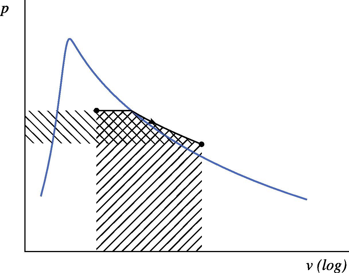
5.4.4 Processes at constant temperature¶

It is possible to heat or cool a liquid-vapor while maintaining its temperature constant (figure 5.18). A process at constant temperature is called an isothermal process.

When the fluid is in a mix of phases (inside of the saturation curve), the constant temperature process also occurs at constant pressure, as described in section §5.4.2 above. In order to quantify the energy transfers, we only need to refer to equations 5/9 and 5/10.

However, as soon as we cross the saturation curve, things change. Once the saturation is reached, the pressure starts to decrease, and we do not have an analytical way to describe this process.

The consequence is that for now, we cannot quantify the work and heat involved when evolving steam at constant temperature! We must wait until chapter 8, where we will use the concept of entropy to tackle the problem.

Figure 5.18:A constant-temperature (isothermal) process undergone by a liquid-vapor. In a closed system (left), the gas is allowed to do work on a piston while being heated, and conversely, work is done on it when cooling. In an open system (right), the same manipulations are carried out continuously.

Diagram CC-by-sa Olivier Cleynen

Figure 5.19:Expansion (heating) at constant temperature of a liquid-vapor, represented on a pressure-volume diagram.

Diagram CC-0 Olivier Cleynen

Example 5.11

How much work and heat are required to slowly heat $2 kg (4.41 lb)$ of saturated liquid water at constant temperature $(130^{\circ}C = 266 ^{\circ} F)$ , until its volume reaches $1 m^{3}(220 imp gal)$ ?

We first observe the final state. The final volume will be $v_{2}= \frac{V_{2}}{m} = 0.5 m^{3}kg^{-1}$ , which is less than $v_{V}$ at our temperature. Therefore, at the end of the heating process, the water will still be partially liquid.

The process will also occur at constant pressure (at the saturation pressure, $p_{\mathrm{sat}130^{\circ}C}= 0.270 28 MPa)$ . The calculation is exactly the same as for example 5.10 p. 133. We obtain a dryness fraction of 0.749, the work (done) is $W_{1\rightarrow 2}= -269.7 kJ$ , and a heat (received) amounts to $Q_{1\rightarrow 2}= +3256.2 kJ$ .

As long as we are in a liquid-vapor mixture (inside the saturation curve), constant temperature = constant pressure. No problem.

Example 5.12

We revisit the same question as in Example 5.11 above with a larger final volume: $2 m^{3}(440 imp gal)$ . How much heat and work are needed?

We cannot yet answer this question! The final specific volume exceeds $v_{V}$ and towards the end of the process, the pressure decreases (figure 5.19).

We could quantify the energy $u_{2}$ by interpolating between the rows and columns of Steam Table 1 (by looking for a volume $v_{2}$ at $130^{\circ}C)$ , which would be imprecise and cumbersome. However, even if we quantified $\Delta u = u_{2}- u_{1}$ , we would be unable to determine the share of work and heat within: both the pressure and volume change, and we are missing a relationship between them to carry out the integral $\int pdv$ .

With the ideal gas model, we could write that $pv =$ cst. at constant temperature, and thus calculate the work during expansion. But with a liquid-vapor mixture, this no longer works.

In chapter 8 (entropy), we will be able to use the brilliant concept of entropy to answer this question.

5.4.5 Reversible adiabatic processes¶

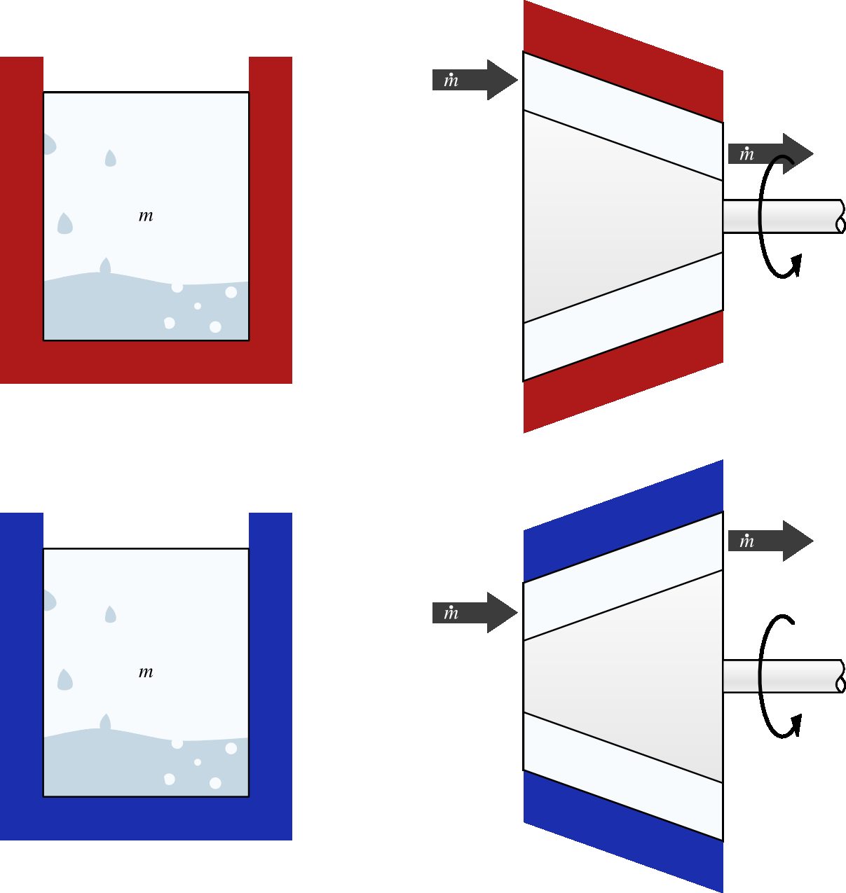
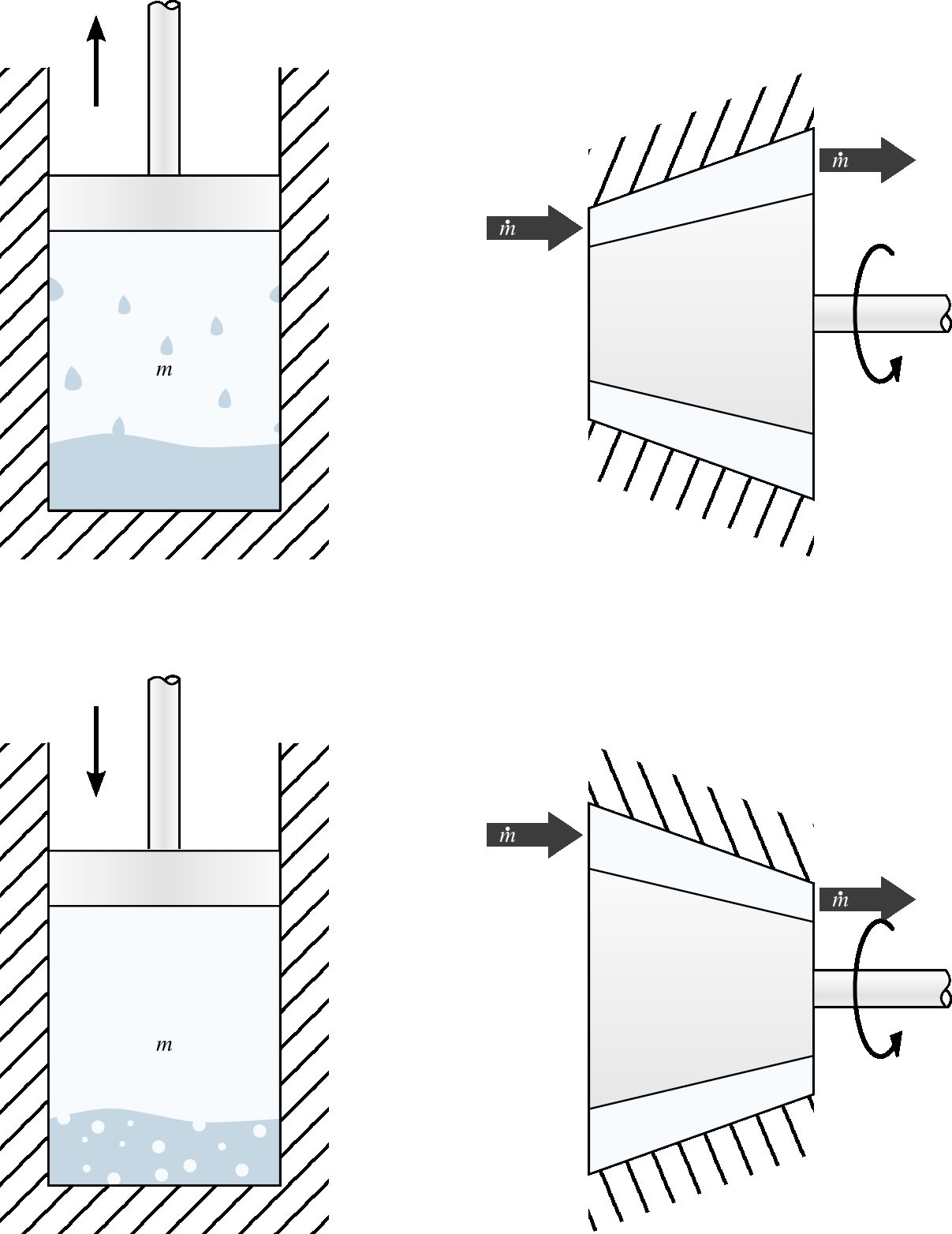
An adiabatic process is a process during which there is no heat transfer (figure 5.20). This can be achieved by covering the container or the duct with a thick layer of thermal insulator.

A reversible adiabatic process is carried out infinitely slowly. For this to happen, a piston in a cylinder will have to be moved infinitely slowly, and a steady-flow turbine will have to be infinitely long. Adiabatic processes serve as a reference, a theoretical goal, to quantify the performances of real turbines, which we will study in chapter 9.

Just like for an ideal gas, the temperature necessarily varies in such a process, since the work is non-zero. It is also noted that the curves of reversible adiabatic processes plotted on a pressure-volume diagram always intersect the saturation curve. In other words, dry steam expanded slowly without heat transfer will, sooner or later, be led to condense. This fact will have significant consequences in chapter 9 (steam power cycles).

Figure 5.20:A reversible adiabatic (isentropic) process undergone by a liquid-vapor. In a closed system (left) as well as in an open system (right), the enclosure is perfectly insulated, so that there is no heat transfer, even if its temperature varies.

Diagram CC-by-sa Olivier Cleynen

In any adiabatic process, the heat transfer is zero:

q_{1\rightarrow 2}= 0

(5/15)

for any adiabatic process.

The work is therefore simply expressed as:

w_{1\rightarrow 2}= \Delta u

(5/16)

for any adiabatic process in a closed system;

Figure 5.21:Reversible adiabatic expansion of a liquid-vapor, represented on a pressure-volume diagram.

Diagram CC-0 Olivier Cleynen

w_{1\rightarrow 2}= \Delta h

(5/17)

for any adiabatic process in an open system.

How to quantify this $\Delta u$ or $\Delta h$ ? Let’s consider the example of an adiabatic expansion, starting from 40 bar and $500^{\circ}C$ . We try to extract the maximum work from the steam before releasing it at atmospheric pressure $(1 bar)$ .

• If the expansion is completely irreversible (very abrupt), then the work is zero. The steam is released with the same amount of energy $(u, h)$ as at the inlet.

• The slower the expansion, the more work we receive.

• The best case – the maximum work – corresponds to a reversible adiabatic expansion (infinitely slow).

Unfortunately, we are still unable to quantify this maximum amount of work! To do this, we would need to be able to quantify the energy within the steam while it expands. We knew how to do this last chapter with an ideal gas (and the daunting relationships of the type $(T_{1}/T_{2})^{1/\gamma -1}= …)$ , but we do not have such a tool with liquids/vapors.

Later, in chapter 8 (entropy), we will see that a reversible adiabatic process occurs at constant entropy (which is why we will call these processes isentropic), and we will use this phenomenal tool to answer these questions.

5.4.6 Arbitrary processes¶

One must keep in mind that in practice, the properties of a liquid-vapor can be arbitrarily changed (figure 5.22), just like with a gas.

We have focused on four specific processes, because each plays an important role, for physicists and engineers, in the design of thermal machines. By cleverly controlling heat and work transfers, of course, we can change the fluid properties any way we would like.

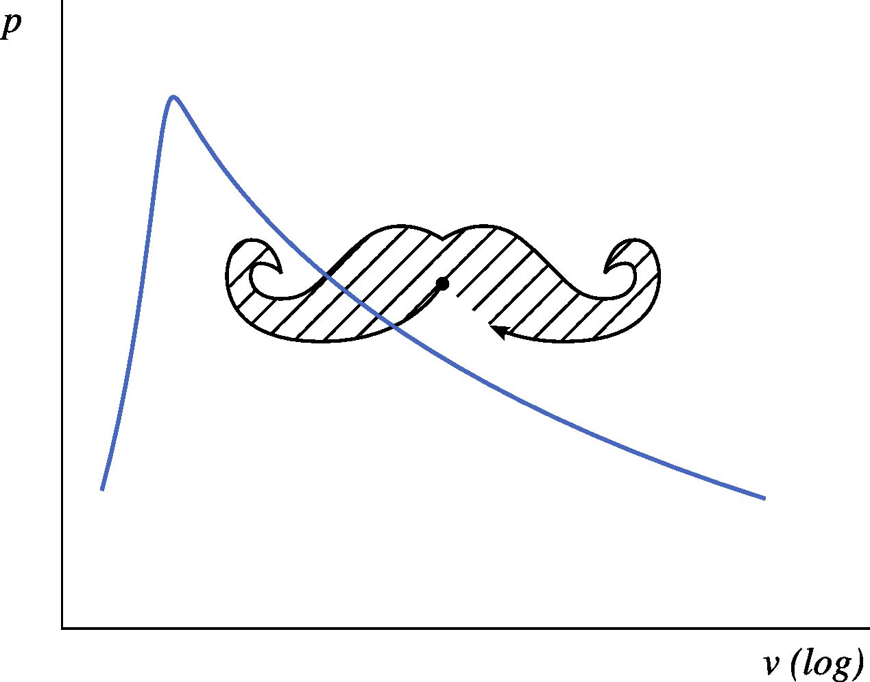
Figure 5.22:A completely arbitrary process undergone by a liquid-vapor represented on a pressure-volume diagram. In addition to a deplorable sense of humor, such a process requires an extremely complex combination of heat and work transfers, which the student is invited to imagine.

Diagram CC-0 Olivier Cleynen

A Bit of History

The Horsepower

We traditionally associate the word engine with automobile propulsion: machines running on air and gasoline. However, the very first engines were quite different. Heavy, slow, incredibly large, running on coal and water, they were only used to pump water.

Let’s go back to the beginning of the 19th century. At that time, Europe was heated by coal, which was extracted with great difficulty from constantly flooded mines. The water was removed by working horses through a primitive pumping mechanism. The first engines were installed to replace these horses – but they were hardly less expensive, and required just as much attention!

For these engines, water is an excellent choice for a working fluid. When steam at moderate pressure is cooled (for example by mixing it with cold liquid water), it condenses and its pressure drops abruptly (figure 5.23). This is an opportunity to drive a piston that, subjected to atmospheric pressure on its other side, can supply work. Thus, one could almost speak of “implosion engines”, since they make the atmosphere work on a cylinder of depressurized steam to produce work.

With this operating mode, the pressure difference obtained reaches a maximum of 1 bar, and the pace is lamentably slow. But these machines operated at reasonable temperatures and pressures, and the operators lacked neither coal nor water. The level of development of metallurgy (cylinders were made of copper, by hand) and mechanical technology (valves had to be successively opened and closed by hand, one by one, to let the engine operate) meant that these engines could only operate with very low pressures.

$Cross-section diagram of one of the first steam engines (Newcomen engine, $\sim 1720)$. The condensation caused by water injection into the cylinder led to a drop in internal pressure.$

Figure 5.23:Cross-section diagram of one of the first steam engines (Newcomen engine, $\sim 1720)$ . The condensation caused by water injection into the cylinder led to a drop in internal pressure.

Engraving by Newton Henry Black & Harvey Nathaniel Davis, published in 1913 (public domain)

It is a young employee of the University of Manchester who first realized the tremendous development potential of the steam engine. By studying a scale model of an engine owned by the university, he made a series of modifications that doubled its efficiency.

The first and most important of these modifications was to separate in space the heating and cooling phases of the steam. Previously, condensation by injection of cold water also lowered the temperature of the metallic piston and cylinder, which had to be heated again at each cycle, with a significant energy cost. Now instead, the steam was cooled in a chamber maintained at low temperature by immersion in water (figure 5.24), while the engine cylinder was kept at a high temperature above the boiler.

Figure 5.24:The Boulton & Watt engine with separate condensation and double-acting piston.

Engraving by Robert Henry Thurston (1878, public domain)

The second modification consisted of exploiting the two faces of the piston. By using a system of pipes controlled by valves, it became possible to increase the pressure difference driving the piston movement. While the steam condensed at $0.2 bar (2.9 psi)$ on one side, the other face now met steam pressurized at $1.4 bar (20.3 psi)$ . Not only was the work done during each piston movement greater, but also the speed (and thus the power) was doubled, since the piston was providing work in both the upward and downward movements.

Finally, a series of mechanical devices reduced the attention that had to be paid to the formidable machinery thus assembled. A large flywheel maintained speed, valve openings were mechanically linked to the engine’s advancement, and the centrifugal ball governor, a technology imported from water mills, prevented engine runaway or stalling (figure 5.25).

Figure 5.25:The ball governor, a mechanism originating from windmills and integrated into steam engines by James Watt.

Engraving by R. Routledge (1900, public domain)

The young laboratory assistant, who went by the name of James Watt, found fortune by partnering with a cannon manufacturer and expert coppersmith, Matthew Boulton. The rest is history: Boulton & Watt captured the lion’s share of the emerging market for heat engines.

Their success, unfortunately, would come much less from the technological innovations they brought than from the high-profile lawsuits they led to monetize them. Indeed, the two partners excelled in political connections and were at home in the peculiar world of patents and the royalties that result from them. The two Scotsmen in top hats, for example, received a percentage of the coal savings generated by the machines they sold across the country. And it would take nearly fifteen years before the legal possibility, in the United Kingdom, to use the “expansive power of steam” became finally open to everyone, a process deviously patented by the two partners!

Regardless, the General Conference on Weights and Measures assigned the unit watt to power in the si system in 1960. It then dethroned the horsepower $(hp)$ ... a unit introduced by the very James Watt nearly a century earlier, while he was comparing his machines with the draft horses they were to replace.

$1 hp_{\mathrm{imperial}}\equiv 33 000 ft lb_{f}\min ^{-1} = 745.6999 W$

Problems¶

The properties of water are tabulated in Steam Tables 1, 2, and 3 (see Appendix A1 p. 305)

Exercise 5.1

Temperature and Boiling Pressure A student is traveling on a commercial flight and is served a hot drink by the cabin crew (figure 5.26); the drink is almost boiling. S/he measures the temperature to be $190.8 ^{\circ} F (88.2^{\circ}C)$ . 1. What is the pressure in the cabin? The aircraft undergoes rapid depressurization and the cabin pressure equalizes with the local atmospheric pressure $(0.175 kg_{f}/cm^{2}$ or $17.2 kPa)$ . The student puts on their oxygen mask and unpleasantly notices that the drink, which is cooling down, has started to boil. 2. At what temperature will the boiling stop? Photo CC-by by Flickr User:notbrucelee

Answer

Interpolating between $T_{\mathrm{sat}.}= 85^{\circ}C$ and $T_{\mathrm{sat}.}= 90^{\circ}C$ in Steam Table 2, we obtain $p_{\mathrm{sat}.}= 0.67 bar$
Interpolating between $p_{\mathrm{sat}.}= 0.016 MPa$ and $p_{\mathrm{sat}.}= 0.018 MPa$ in Steam Table 3, we obtain $T_{\mathrm{sat}.}= 56.8^{\circ}C = 134.2 ^{\circ} F$ (yuck!)

Figure 5.26:An aerial hot drink with an unidentified taste

Exercise 5.2

Evaporation of Water 1. How much heat is needed to completely evaporate a pot of water (figure 5.27)? The container contains $2.5 L (0.66 US gal)$ of water at $50 ^{\circ} F (10^{\circ}C)$ , and the ambient atmospheric pressure is $1 bar (14.5 psi)$ . 2. Draw the process qualitatively (that is, without showing numerical values) on a temperature-volume diagram, showing the saturation curve. 3. The water is heated with an electric heating plate of $1500 W$ . How long does it take to vaporize the water, and what is the cost incurred by the experiment? The operator charges 0.15AC per $kW h$ and the losses from the plate to the room are around $10 \%$ . Photo CC-by by Indi Samarajiva

Answer

To heat up the water until the boiling point (B) then complete evaporation (C): $Q_{\mathrm{A}\rightarrow \mathrm{C}}= m(q_{\mathrm{A}\rightarrow \mathrm{B}}+ q_{\mathrm{B}\rightarrow \mathrm{C}}) = \frac{V_{\mathrm{A}}}{v_{\mathrm{A}}} (h_{L 0.1 MPa}-h_{\mathrm{A}}+h_{LV 0.1 MPa}) = +6582 kJ$ .
$\Delta t = \frac{Q_{\mathrm{A}\rightarrow \mathrm{C}}}{\dot{Q}_{\mathrm{average}}} = 1 h 21 \min$ with a cost of 0.29AC.

Figure 5.27:An ordinary physics experiment

Exercise 5.4

High-Pressure Steam Generation An industrial chemical process requires a steam flow rate of $2 kg s^{-1}(4.41 lb/s)$ at $6 bar$ and $875^{\circ}C (87 psi$ and $1607 ^{\circ} F)$ . The machine responsible for providing this steam is fed by a pressurized liquid water pipeline at $10^{\circ}C$ and $6 bar (50 ^{\circ} F$ and $87 psi)$ . 1. What power in the form of work and heat is required to generate this steam flow? 2. Draw the process undergone by the water on a pressure-volume diagram, qualitatively (that is, without showing numerical values), showing the saturation curve.

Answer

Reading in Steam Table 1 @ $p_{\mathrm{A}}= 0.6 MPa$ , $h_{\mathrm{A}}= 42.6 kJ kg^{-1}$ . Interpolating between 800 and $900^{\circ}C$ in this table, we obtain $h_{\mathrm{B}}= 4336.6 kJ kg^{-1}$ . Thus with equation 5/10, $\dot{Q}_{\mathrm{A}\rightarrow \mathrm{B}}= \dot{m}\Delta h = +8.59 MW$ . $\dot{W}_{\mathrm{A}\rightarrow \mathrm{B}}= 0 W$ (5/9).

Exercise 5.5

Everything Depends On the Valve A student decides to maintain a balanced diet, and to do so, cooks food in a pressure cooker (figure 5.28). The valve of the pressure cooker is a small metal cylinder that is partly hollowed out, and sits freely on top of a small vertical exhaust pipe on the lid. The valve weighs $0.476 lb (216 g)$ ; it is placed on an exhaust pipe with a diameter of $5 mm (0.197 in)$ . The ambient atmospheric pressure is $1.122 kg_{f}/cm^{2}(1.1 bar)$ . 1. At which temperature does the pressure cooker allow the student to food their cook? 2. What temperature and pressure could a person generate inside the pressure cooker by pressing on the valve? How could an accident be then prevented? Photo CC-by-sa by Commons User:rama

Answer

$p_{\mathrm{inner}}= p_{\mathrm{valve}}+ p_{\mathrm{atm}.}= \frac{F_{\mathrm{weight}}}{S_{\mathrm{outlet}}} + 1 bar = 2.0797 bar$ . Interpolating in Steam Table 2, $T_{\mathrm{sat}.p=2.0797 bar}= 121.37^{\circ}C = 250.47 ^{\circ} F$ .

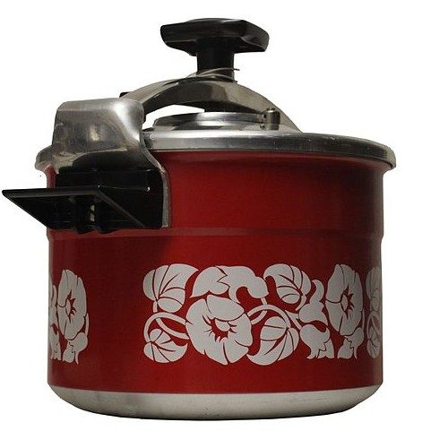
Figure 5.28:A pressure cooker, in which the increased pressure results in higher boiling temperature and thus faster cooking. It is affectionately known as a *cocotte minute* in France.

Exercise 5.6

A First Steam Engine An engineer conducts an experiment with water vapor, aiming to develop a very simple, small steam engine (figure 5.29). S/he puts $2 L (0.44 imp gal)$ of liquid water at $20^{\circ}C$ into a large cylinder. The water is compressed to 2 bar by a piston. S/he then heats the water, and the piston moves while maintaining constant pressure, until the volume reaches $300 L (66 imp gal)$ . 1. Draw the process qualitatively (that is, without showing numerical values) on a pressure-volume diagram, showing the saturation curve. 2. What was the amount of work done? 3. How much heat had to be supplied? 4. What would be the transfers of work and heat if the expansion were continued until $4500 L (990 imp gal)$ ? Diagram CC-0 by Olivier Cleynen

Answer

$W_{\mathrm{A}\rightarrow \mathrm{B}}\approx 0$ (equation 5/11); with $m = \frac{V_{\mathrm{B}}}{v_{\mathrm{B}}}$ and $v_{\mathrm{D}}= \frac{V_{\mathrm{D}}}{m}$ , we calculate $W_{\mathrm{B}\rightarrow \mathrm{D}}= -mp_{\mathrm{cst}.}(v_{\mathrm{D}}-v_{\mathrm{B}}) = -59.6 kJ$ (equation 5/7). 3) With $v_{\mathrm{D}}$ we calculate the dryness fraction $x_{\mathrm{D}}\approx \frac{v_{\mathrm{D}}}{v_{V0.2MPa}} = 0.1697$ . Thus, $Q_{\mathrm{B}\rightarrow \mathrm{D}}= m(h_{\mathrm{D}}- h_{\mathrm{B}}) = m(h_{L}+ x_{\mathrm{D}}h_{LV}-h_{\mathrm{B}}) = +1585.2 kJ$ (equation 5/8), so twenty-five times more...
The relationships are identical and yield $W_{\mathrm{B}\rightarrow \mathrm{E}}= -899.6 kJ$ and $Q_{\mathrm{B}\rightarrow \mathrm{E}}= +7694.3 kJ$ (the efficiency jumps from 3.8 to $11.7 \%$ ... there is a lead to follow here...)

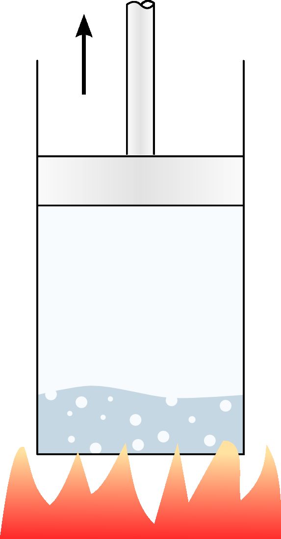
Figure 5.29:A very basic concept of a steam engine

Exercise 5.7

Pumping Water A pump is installed to draw liquid water at $5^{\circ}C$ located up from a lower tank (figure 5.30). 1. Up to what height $\Delta z$ can the pumping be done? 2. How could we change the setup to pump water to a greater height? below. The first observation of the height limit calculated in this problem was made in 1630 by Giovanni Battista Baliani. Sketch CC-0 by Olivier Cleynen

Answer

Hydrostatic pressure in the pipe depends on height $(\Delta p = \rho g\Delta z)$ . When the pressure at the pump goes below $p_{\mathrm{sat}.}$ , the water starts boiling. For $\Delta p_{\mathrm{boiling}}= 9.9127 \times 10^{4}Pa, \Delta z_{\mathrm{boiling}}= 10.1 m$ .
One can do better than heating up the tank...

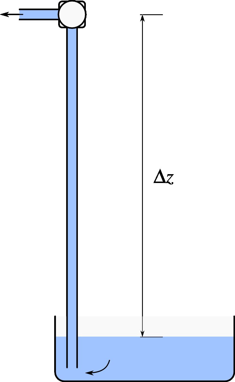
Figure 5.30:Water pumping from a reservoir located below. The first observation of the height limit calculated in this problem was made in 1630 by Giovanni Battista Baliani.

Exercise 5.8

Steam Turbine On a Portable Power Plant A company is developing a small steam power plant that can be carried in a standard-sized shipping container. Once connected to an external boiler, it is capable of converting heat from unrefined fuels (such as wood, paper, or coal) into electricity with a relatively high efficiency. Within this power plant, the turbine is adiabatic and receives $5 t/h (11 023 lb/h)$ of steam at 90 bar and $510^{\circ}C$ from the boiler. The outlet pressure is barely above atmospheric pressure (we will take $1 bar)$ . An engineer predicts, as we will also be able to do after chapter 8 (entropy), that the outlet specific internal energy of the steam will then be $2676.6 kJ kg^{-1}$ . The turbine is mechanically connected to a power generator with an efficiency of $85 \%$ . 1. What is the power output of the generator? At the other end of the container, an electric pump (the only other mechanical element in the plant) collects the condensed water in saturated liquid state $(1 bar)$ and increases its pressure back to 90 bar to feed the boiler. It is assumed that during pumping, the specific volume of water varies negligibly, and that the compression is reversible. 2. What is the power required to power the pump?

Answer

In A in Steam Table 1 we interpolate at $9 MPa$ between 500 and $600^{\circ}C$ to obtain $h_{510^{\circ}C\&90 bar}= 3412 kJ kg^{-1}$ . The same is done in B where $u_{\mathrm{B}}> u_{V1 bar}(h_{\mathrm{B}}= 2899.4 kJ kg^{-1})$ . Finally $\dot{W}_{\mathrm{electrical}}= \eta _{\mathrm{conversion}}\dot{m}\Delta h = -605.8 kW$ . $2)\dot{W}_{\mathrm{pump}}=\dot{m}\int vdp \approx \dot{mv}_{L}\Delta p = +12.9 kW$ .

Exercise 5.9

The Crushed Barrel In order to perform a physics demonstration, a group of students bring water to boil at ambient pressure in a steel drum. The drum’s capacity is $55 US gal (208 L)$ and it is $34.6 in (88 cm)$ high. The barrel is removed from the heat source and hermetically sealed. The purpose of the operation is to observe the barrel being crushed by the atmosphere due to the change of internal pressure as the contained water condenses. 1. Which pressure can be generated inside the barrel by letting it cool down? 2. What would be the vertical force exerted on the upper wall of the barrel at that point? Some more challenging questions: 3. There are $5 L (1.32 US gal)$ of liquid left at the bottom of the barrel when the lid is closed. What is the steam dryness fraction? 4. How much steam has condensed during cooling? 5. How much heat had to be removed in order to reach the final pressure?

Answer

If we attain $T_{\mathrm{B}}= 30^{\circ}C$ with constant volume, then $p_{\mathrm{inside} \min.}= p_{\mathrm{sat}.30^{\circ}C}= 0.004 247 MPa$ . In that case, $\Delta p_{\max}= -9.575 \times 10^{4}Pa = -13.89 psi$ ;
$F_{\max}= \Delta p_{\max}S_{\mathrm{lid}}= -22.6 kN = 5081 lb_{f}$ (the barrel will of course be crushed before that);
$x_{\mathrm{A}}= 0.024 39, x_{\mathrm{B}}= 1.288 \times 10^{-3}$ ;
$m_{\mathrm{condensed}}= 0.113 52 kg = 0.25 lb$ ;
$Q_{\mathrm{A}\rightarrow \mathrm{B}}= -1.669 MJ$ .

Exercise 5.10

Newcomen Engine In their time, around 1720, Newcomen engines (figure 5.23) were at the forefront of technology. Slightly overheated steam $(1 bar, 250^{\circ}C)$ was injected into a large cylinder (height $1 m$ , diameter $1.5 m)$ . This steam was then cooled (by allowing a small amount of liquid water at atmospheric pressure and temperature to enter), maintaining the internal pressure at 0.1 bar. The piston would then descend, providing work. The water available to the engine was at $1 bar, 10^{\circ}C$ . 1. Plot the process on a pressure-volume or temperature-volume diagram, showing the saturation curve. 2. How much heat must be supplied to fill the cylinder with steam before the descent can be performed? 3. How much work is supplied by the engine during the piston’s descent? Hint: Consider the work done by the atmosphere on the outer face of the piston. 4. What is the efficiency of the engine, if friction and all other heat losses are neglected? Newcomen, the first true success in steam power. Engraving C. L. Moll (1873, public domain)

Answer

Reading Steam Table 1 gives us $h_{\mathrm{A}}= 42.1 kJ kg^{-1}$ . Through interpolation we obtain $h_{\mathrm{B}}= 2975 kJ kg^{-1}$ and $m = \frac{V_{\mathrm{B}}}{v_{\mathrm{B}}} = 0.7354 kg$ . Thus we calculate $Q_{\mathrm{A}\rightarrow \mathrm{B}}= m\Delta h = +2154 kJ$ (equation 5/8).
While calculating $m$ we already obtained $v_{\mathrm{B}}= 2.406 m^{3}kg^{-1}$ . Thus $W_{\mathrm{piston}\rightarrow \mathrm{shaft}}= W_{\mathrm{atm}.\rightarrow \mathrm{piston}}+ W_{\mathrm{piston}\rightarrow \mathrm{steam}}= m(p_{\mathrm{C}}-p_{\mathrm{ext}.})(v_{\mathrm{D}}-v_{\mathrm{C}}) = -159 kJ$ .
$\eta \equiv \frac{Q_{\mathrm{supplied}}}{W_{\mathrm{useful}}} = 7.38 \%$ (realistic value).

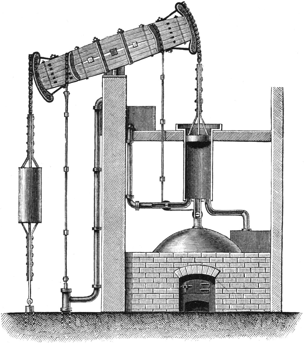
Figure 5.31:The ingenious atmospheric engine by Newcomen, the first true success in steam power.

Exercise 5.11

Condenser of a Steam Power Plant In a high-power electric power plant, the condenser is responsible for recovering water at the output of the turbines and removing energy from it, so that it may return to the liquid state and re-enter the pumps $\rightarrow$ boilers $\rightarrow$ turbines circuit. The water from the system $(180 t/h)$ arrives at 0.5 bar with a specific volume of $3.1247 m^{3}kg^{-1}$ ; it must leave at the same pressure, in a saturated liquid state. In order to extract heat from the water in the power plant, the condensers use a secondary water circuit directly from a river, where water is drawn at $10^{\circ}C$ . In order to reduce the ecological impact of the power plant, the goal is to discharge the secondary water into the river at a temperature no higher than $35^{\circ}C$ . 1. What flow rate of secondary water should be drawn from the river? 2. In order to limit heat discharge into the river, where (and how) is the condenser heat also discharged in practice?

Answer

$x_{\mathrm{A}}= 96.44 \% \& x_{\mathrm{B}}= 0$ ; thus $\dot{Q}_{\mathrm{A}\rightarrow \mathrm{B}}= -111.13 MW$ , which is the reason why we need $m_{\mathrm{secondary}}\ge 1062.4 kg s^{-1}$ or $2342.2 lb/s$ . 2) Into the atmosphere, through the secondary water which is released through the large towers...

Exercise 5.12

Aircraft Catapult On an Aircraft Carrier An aircraft catapult is mounted on a military ship (figures 5.32 and 5.33). It consists of a steam reservoir connected to a long cylinder, in which a piston slides to propel the aircraft during takeoff. At the beginning of the catapult launch, the steam is at 140 bar and $700^{\circ}C$ . After a brief run of $50 m$ , the aircraft has left the deck and the steam is at 4 bar and $410^{\circ}C$ . 1. How much energy did the catapult provide to the aircraft per kilogram of steam? 2. What must be the diameter of the piston and the total mass of steam, for the thrust provided to the aircraft to always exceed $2.5 t_{f}(5512 lbf)$ ? (And a question which we can not yet answer: what is the maximum amount of energy that the catapult could have supplied to the aircraft by allowing the steam to expand?) Photo by Geoffrey Lewis, U.S. Navy (public domain) Photo CC-by-sa by Jean-Michel Roche, Netmarine.net

Answer

$\Delta u = -433.1 kJ kg^{-1}(= w_{\mathrm{A}\rightarrow \mathrm{B}}$ if we suppose that the process is adiabatic); 2) $D_{\min.}= 32.26 cm$ (care must be taken to take atmospheric pressure into account); $m = \frac{V_{\max}-V_{\min}}{v_{\max}-v_{\min}} = 5.243 kg$ . Nota: the data given in this problem is hypothetical, for lack of reliable published data.

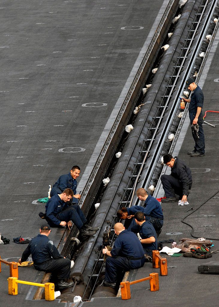
Cylinder of a steam catapult from the USS Abraham Lincoln — Figure 5.32:Cylinder of a steam catapult from the *USS Abraham Lincoln*

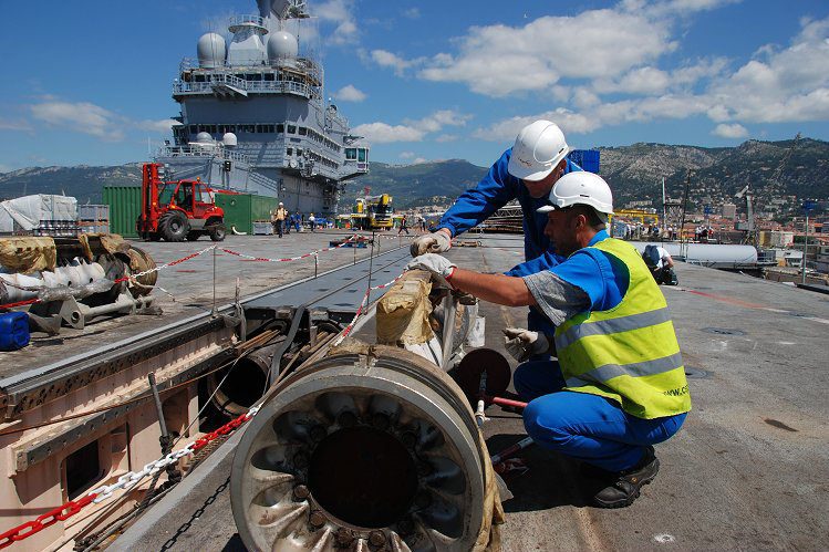
Piston of a steam catapult from the aircraft carrier Charles de Gaulle. — Figure 5.33:Piston of a steam catapult from the aircraft carrier *Charles de Gaulle*.

Exercise 5.13

Turbine of a Nuclear Power Plant In a nuclear power plant, the electricity generator is driven by a steam turbine (figure 5.34). Most of the steam (heated by the nuclear reactor) passes through the entire turbine. However, in the middle of the turbine, a steam bleed is carried out. It allows, on one hand, to heat the water in another part of the circuit (§9.4.5), and on the other hand, to precisely control the mass flow rate in circulation. The total flow rate at the inlet is $317 t/h$ of steam. We measure the following steam properties: Inlet: 120 bar; $565^{\circ}C$ Extraction: 10 bar; $250^{\circ}C$ ; $1.2 kg s^{-1}$ Outlet: 1 bar; $115^{\circ}C$ What is the shaft power of the turbine? akovo nuclear power station $(\sim 1 GW$ plant power), in maintenance (top) and during installation (bottom). Photos 1 and 2 CC-by-sa The Centre of the Public Information Balakovo NPP

Answer

$W_{\mathrm{turbine}}= -71 MW$ .

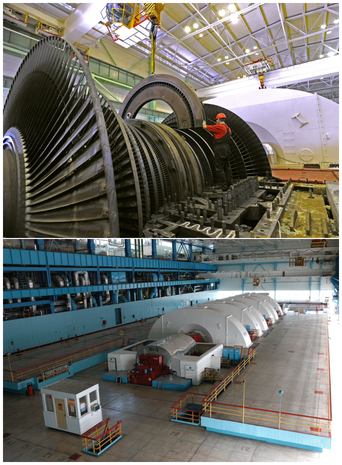
One of the turbines at the Russian Balakovo nuclear power station plant power), in maintenance (top) and during installation (bottom). — Figure 5.34:One of the turbines at the Russian Balakovo nuclear power station $(\sim 1 GW$ plant power), in maintenance (top) and during installation (bottom).

Footnotes¶

The term incompressible, a true false friend for the student, does not mean that the pressure is constant or uniform. It merely means that the specific volume $v$ , and thus with it the density $\rho$ , remains constant.
↩
Strictly speaking, the mixture is called saturated liquid-vapor mixture, since it consists of saturated liquid and saturated vapor. It can also be named wet vapor.
↩

Introduction¶

5.1 Evaporation and Condensation¶

5.1.1 What is a liquid?¶

5.1.2 Phase changes¶

5.1.3 One way to approach evaporation and¶

condensation¶

5.1.4 Industrial use of water and liquids/vapors¶

5.2 Qualitative Description of Water Properties¶

Properties¶

5.2.1 Limits of the ideal gas¶

5.2.2 The temperature-volume** (T−v)(T-v)(T−v) **diagram¶

5.2.3 The pressure-volume diagram** (p−v)(p-v)(p−v)¶

5.2.4 A student’s false friend¶

5.2.5 Water in everyday life¶

5.3 Quantifying the Properties of Water¶

5.3.1 Subcooled liquid and superheated vapor¶

5.3.2 Saturation points¶

5.3.3 The liquid-vapor mixture¶

5.4 Elementary Reversible Processes¶

5.4.1 What is this chapter section for?¶

5.4.2 Processes at constant pressure¶

5.4.3 Processes at constant volume¶

5.4.4 Processes at constant temperature¶

5.4.5 Reversible adiabatic processes¶

5.4.6 Arbitrary processes¶

Problems¶

5.2.2 The temperature-volume $(T-v)$ diagram¶

5.2.3 The pressure-volume diagram** $(p-v)$ ¶