Within the first-order, paraxial approximation of Gaussian geometrical optics, a spherical surface maps an object point to a real or virtual image point. A sequence of such surfaces can be treated one surface at a time: the image formed by each surface becomes the object for the next, and intermediate objects or images may be virtual. Real optical systems also have aberrations outside this approximation.
Although this procedure is in principle simple, it is nevertheless convenient in Gaussian geometrical optics to introduce the concept of ray vectors and ray matrices to deal with optical systems consisting of several spherical surfaces.
With ray matrices it is easy to derive how the distance of a given ray to the optical axis and its direction change during propagation through an optical system. This in turn can be used to determine the image plane in an optical system for a given object plane.
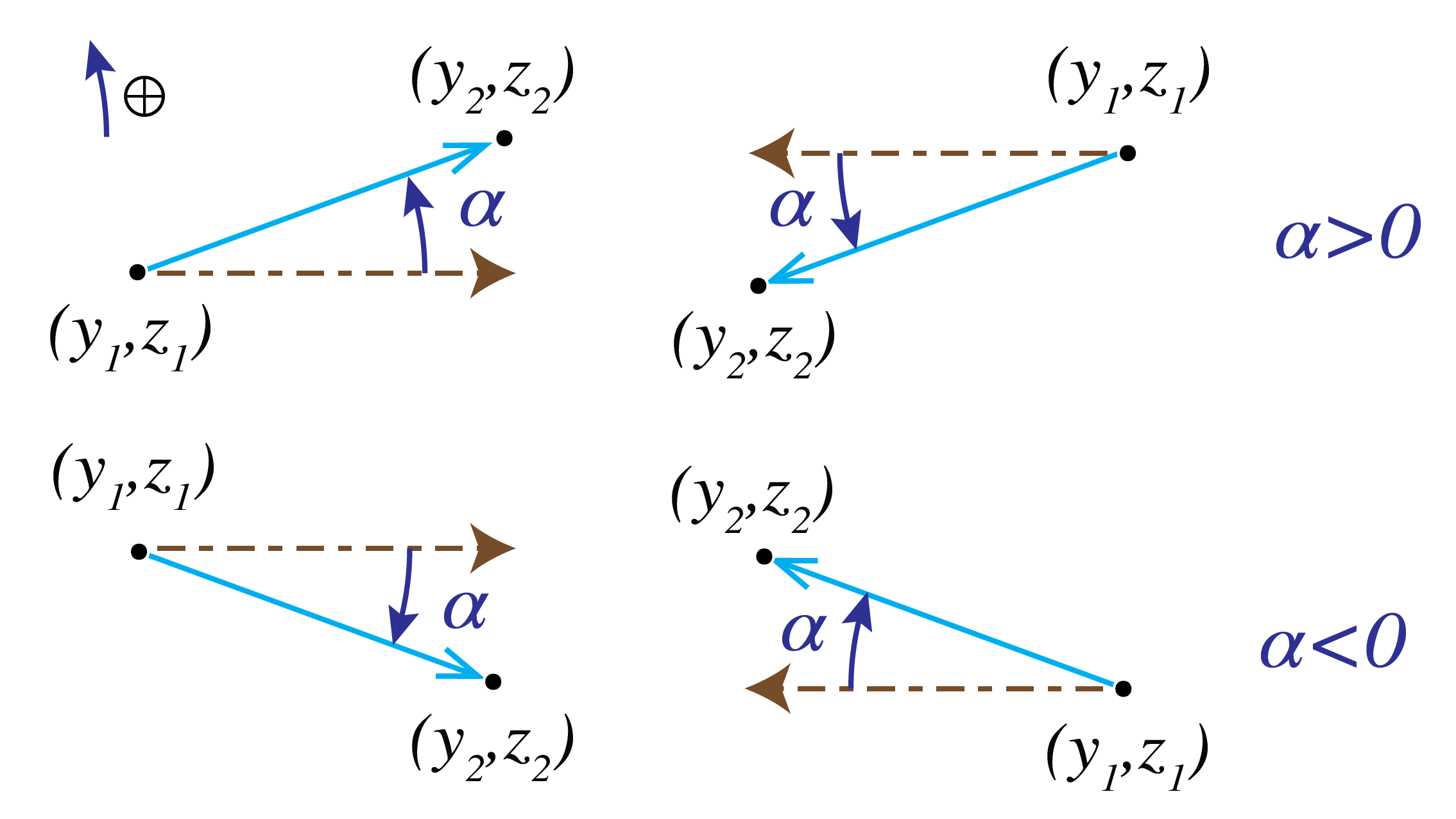
In any plane perpendicular to the z-axis, a ray is determined by the y-coordinate of the point of intersection of the ray with the plane and the angle α with the optical (z)-axis. This angle has a sign and is defined as follows. Let (y1,z1) and (y2,z2) be the coordinates of two points on the ray and let the light propagate from point 1 to point 2. Then we define
Examples of positive and negative α are given in Figure 1. The case z2−z1<0 occurs when a ray propagates in the negative z-direction after it has been reflected by a mirror.
According to the sign convention table in the Geometrical Optics chapter, the refractive index of the ambient medium should after the reflection be taken negative. After a second reflection due to which the ray propagates again in the positive z-direction the refractive index should be chosen positive again.
Figure 1:Sign convention for the ray angle. In the upper two figures α>0 while in the lower two figures α<0.
where n is the local refractive index. The definition with the refractive index as factor in the first element of the ray vector turns out to be convenient.
The ray vectors of a ray in any two planes z=z1, z=z2, with z2>z1, are related by a so-called ray matrix:
The elements of matrix M depend on the optical components and materials between the planes z=z1 and z=z2.
As an example consider the ray matrix that relates a ray vector in the plane immediately before a spherical surface (see the Geometrical Optics chapter for details on spherical interface imaging) to the corresponding ray vector in the plane immediately behind that surface.
Using the paraxial Snell’s law and small-angle approximations from the Geometrical Optics chapter, it
follows
where we have replaced α2 by −α2 in the paraxial Snell’s law equation from the Geometrical Optics chapter, because according to the sign convention, the
angle α2 should be taken
negative.
Because furthermore y2=y1, we conclude
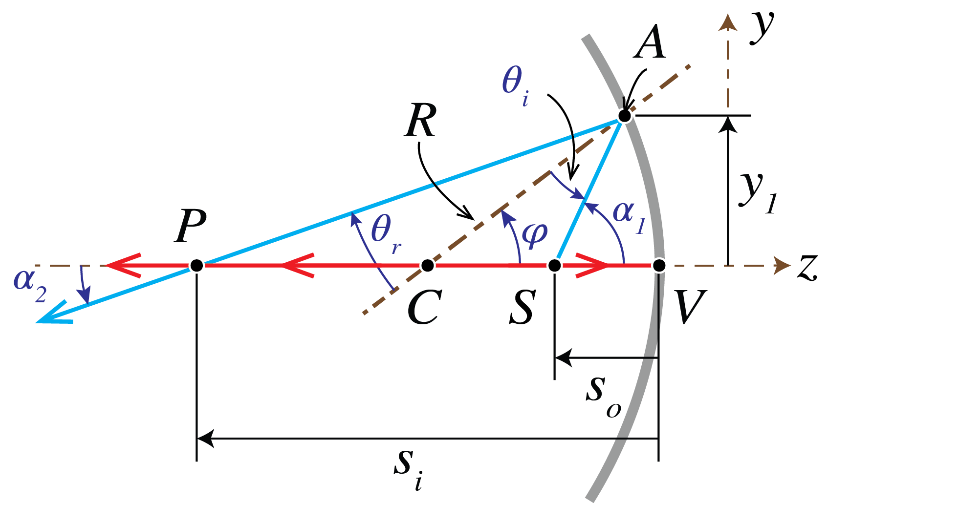
Next we consider a spherical mirror with radius of curvature R.
We will show that the ray matrix between the planes just before and after the mirror is given by:
is the power of the mirror, n1=n but n2=−n, because the convention is used that if a ray propagates from right to left (i.e. in the negative z-direction), the refractive index in the ray vectors and ray matrices is chosen negative. Note that when the mirror is flat: R=∞, the ray matrix of the reflector implies
In the situation drawn in Figure 2, Eq. (1) implies that both α2 and α1 are
positive. By choosing the refractive index negative after reflection,
we conclude from Eq. (13) and Eq. (14):
We now consider the ray matrix when a ray propagates from a plane z1 to a plane z2 through a medium with refractive index n.
In that case we have
α2=α1 and y2=y1+α1(z2−z1), hence
Note that if the light propagates from the left to the right: z2>z1 and hence z2−z1 in the first column and second row of the matrix is positive, i.e. it is the distance between the planes.
For two planes between which there are a number of optical components, possibly separated by regions with homogeneous material (e.g. air), the ray matrix can be obtained by multiplying the matrices of the individual components and of the homogeneous regions. The order of the multiplication of the matrices is such that the right-most matrix corresponds to the first component that is encountered while propagating, and so on.
The matrices here describe meridional rays in a plane containing the optical axis, giving a two-dimensional model. Skew rays do not intersect the optical axis and require a fuller three-dimensional treatment; a skew ray can still be paraxial.
Remarks.
In matrix Eq. (16), z1 and z2 are signed coordinates.
Instead of choosing the refractive index negative in ray vectors of rays that propagate from right to left, one can reverse the direction of the positive z-axis after every reflection. The convention to make the refractive index negative is however more convenient in ray tracing software.
The determinants of the ray matrices Eq. (6),
Eq. (8) and
Eq. (16) are all 1. Since all ray matrices
considered below are products of these elementary matrices, the determinant
of every ray matrix considered is unity.
We apply ray matrices to a lens.
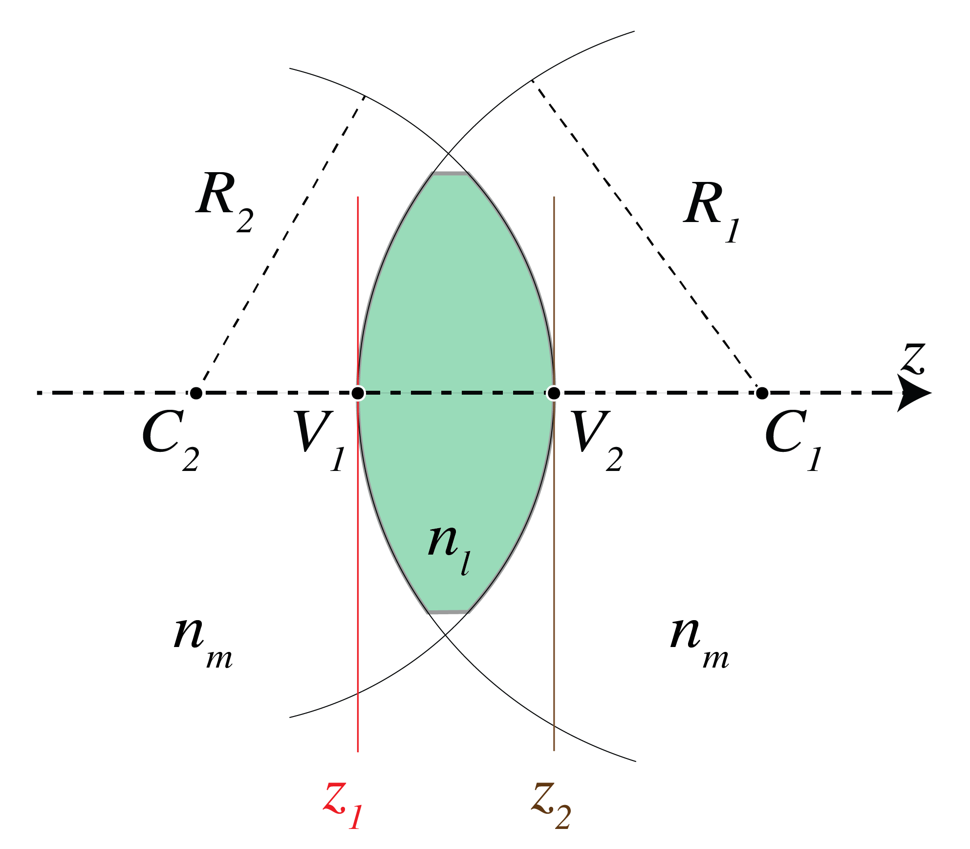
Figure 3 shows a lens with two spherical surfaces. The refractive index of the lens is nl and the refractive indices of the media to the left and right of the lens are n1 and n2, respectively. Let the distance between the vertices be d.
Figure 3:A lens with thickness d. The ray matrix is defined between the planes immediately before and after the lens.
We will first derive the matrix which maps the ray vector in the plane immediately in front of the lens to that in the plane immediately behind the lens. Let
be two vectors in the two planes which correspond to the same ray. The ray is
first refracted by the spherical surface with radius R1 and center C1.
Using Eq. (6) and Eq. (7) it follows that the matrix between the ray
vectors just before and just behind the spherical surface with radius R1 and
center C1 is given by
The ray then propagates over the distance d through the material of which the
lens is made. The matrix that maps ray vectors from the plane inside the lens
immediately behind the left spherical surface to a ray vector in the plane
immediately before the right spherical surface follows from Eq. (16):
Finally, the matrix that maps ray vectors from the plane in the lens immediately before the second spherical surface to vectors in the plane immediately behind it is
Hence the matrix that maps ray vectors in the plane immediately before the lens to ray vectors in the plane immediately behind the lens is given by the matrix product:
is called the power of the lens. It has dimension 1/length and is given in diopter (D), where 1D=m−1. The power can be positive or negative.
The space to the left of the lens is called the object space and that to the right of the lens is called the image space.
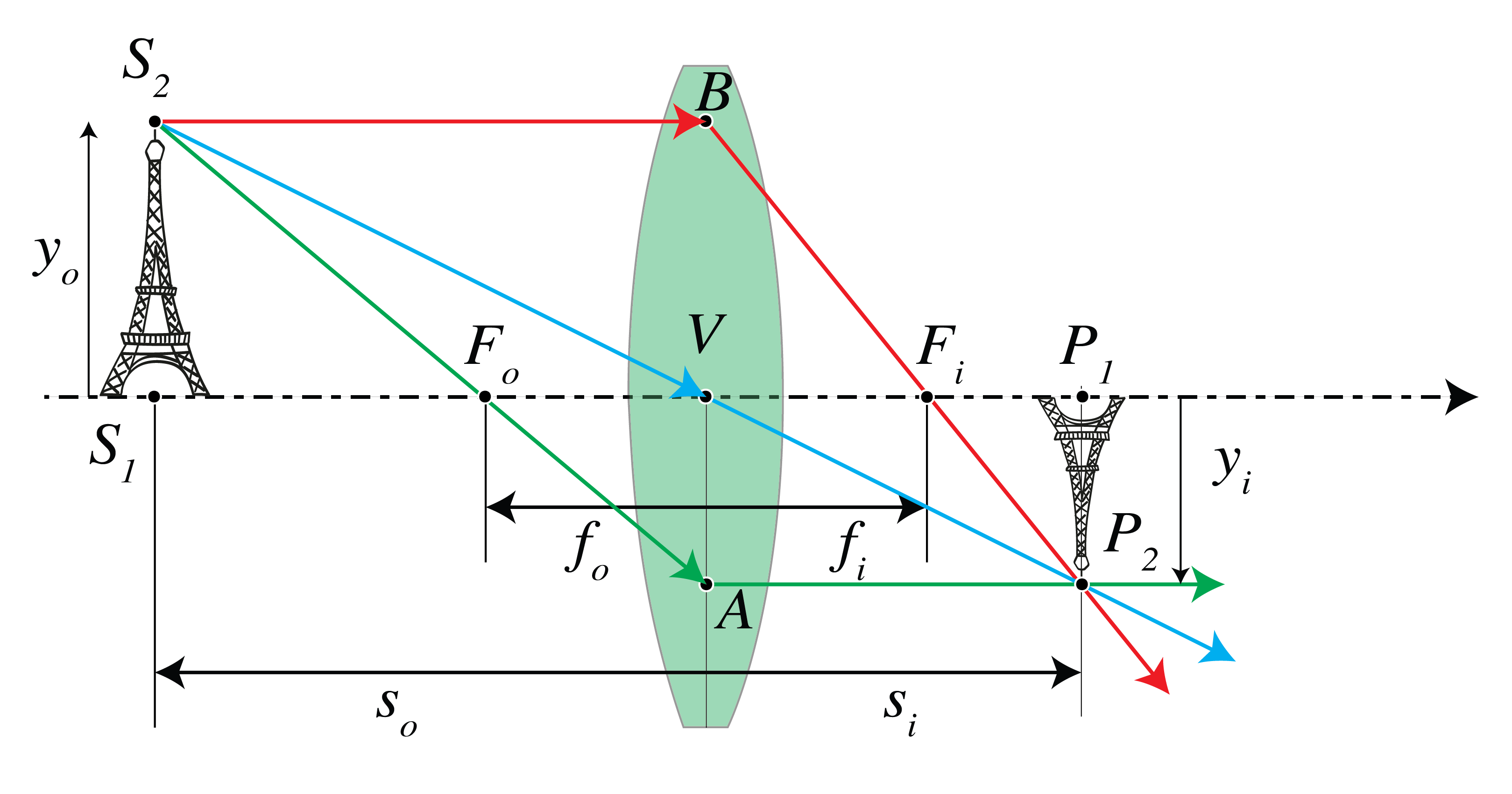
Figure 4:Place a thin lens on the bench, send in a parallel beam, and measure where it crosses the axis — the second focal point of the matrix M derived above. Add an off-axis object ray and recover the imaging relation of the next section.
This power–curvature relation is the lensmaker formula for a thin lens. The origin of the coordinate system is chosen at the common vertex V1=V2.
By considering a ray in medium 1 which is parallel to the optical axis (α1=0) and at height y1, we get n2α2=−Py1 and y2=y1. Hence, when P>0, the angle α2 of the ray has sign opposite to y2 and therefore the ray in image space is bent back to the optical axis, yielding a second focal point or image focal pointFi. Its
z-coordinate fi is:
If the power is positive: P>0, the angle α1 has the same sign as y1, which implies that the ray in object space has intersected the optical axis in a point Fo with z-coordinate: z=fo
The point Fo is called the first focal point or object focal point.
We conclude that when the power P of the lens is positive, fi>0 and −fo>0, which means that the image and object focal points are in the image and object space, respectively, hence they are both real. A lens with positive power is called convergent or positive. It makes incident bundles of rays convergent or less divergent.
A lens with negative power is called divergent and has fi<0, −fo<0. It makes incident rays more divergent or less convergent.
Incident rays which are parallel to the optical axis are refracted away from the optical axis and seem to come from a point in front of the lens with z-coordinate fi<0. Hence the image focal point does not correspond to a location where there is an actual concentration of light intensity, i.e. it is virtual. The object focal point is a virtual object point, because only a bundle of incident rays that are converging to a certain point behind the negative lens can be turned into a bundle of rays parallel to the optical axis.
With the results obtained for the focal coordinates we can rewrite the lens matrix of a thin lens as
We first consider a general ray matrix Eq. (3), Eq. (4) between two planes z=z1 and z=z2 and ask the
following question:
what are the properties of the ray matrix such that the two planes are images of each other, or (as this is also called) are each other’s conjugate?
Clearly for these planes to be each other’s image, we should have that for every point coordinate y1 in the plane z=z1 there is a point with some coordinate y2 in the plane z=z2 such that any ray through (y1,z1) (within some cone of rays) will pass through the point (y2,z2).
Hence for any angle α1 (in some interval of angles) there is an
angle α2 such that Eq. (3) is valid.
This means that for any y1 there is a y2 such that for all angles α1:
is the magnification of the image (this quantity has sign).
To determine the image by a thin lens we first derive the ray matrix between two planes z=z1<0 and z=z2>0 on either side of the thin lens. The origin of the coordinate system is again at the vertex of the thin lens.
This ray matrix is the product of the matrix for propagation from z=z1 to the plane immediately in front of the lens, the matrix of the thin lens and the matrix for propagation from the plane immediately behind the lens to the plane z=z2:
where we have written so=z1 and si=z2 for the z-coordinates of the object and the image.
Because for the thin lens matrix Eq. (34): D=1−z2/fi, it follows by using Eq. (35) that the magnification Eq. (33) is given by
where we have written now yo and yi instead of y1 and y2, respectively.
Remark.
The thin-lens imaging equation can alternatively be derived
by using the single-surface imaging formula from the Geometrical Optics chapter for the two
spherical surfaces of the lens. We first image a given point S by the left
spherical surface using that imaging formula as if the second
surface were absent. The obtained intermediate image P′ is then imaged by the
second spherical surface as if the first surface were absent. P′ can be a real
or virtual object for the second surface. The derivation is carried out in
Problem 2.5.
Analogous to the case of a single spherical surface, an image is called a real image if it is to the right of the lens (si>0) and is called a virtual image when it seems to be to the left of the lens (si<0). An object is called a real object if it is to the left of the lens (so<0) and is a virtual object if it seems to be to the right of the lens (so>0).
For a positive lens: P>0 and hence Eq. (35)
implies that si>0 provided ∣so∣>∣fo∣, which means that the image by a
convergent lens is real if the object is further from the lens than the object
focal point Fo.
The case so>0 corresponds to a virtual object, i.e. to the case of a converging bundle of incident rays, which for an observer in object space seems to converge to a point at distance so behind the lens.
A convergent lens (fi>0) will then make an image between the lens and the second focal point. In contrast, a diverging lens (fi<0) can turn the incident converging bundle into a real image only if the virtual object point is between the lens and the focal point. If the virtual object point has larger distance to the lens, the convergence of the incident bundle is too weak and the diverging lens then refracts this bundle into a diverging bundle of rays which seem to come from a virtual image point in front of the lens (si<0).
Instead of using ray matrices, one can construct the image with a ruler.
Consider the imaging of a finite object S1S2 as shown in Figure 5 for the case that the media to the left and right of the lens are the same. Let yo be the y-coordinate of S2. We have yo>0 when the object is above the optical axis.
Draw the ray through the focal point Fo in object space and the ray through the center V of the lens. The first ray becomes parallel in image space. The latter intersects both surfaces of the lens almost in their (almost coinciding) vertices and therefore the refraction is opposite at both surfaces and the ray exits the lens parallel to its direction of incidence. Furthermore, its lateral displacement can be neglected because the lens is thin. (Of course, this is not correct when the refractive indices to the left and right of the lens are different). Hence, the ray through the center of a thin lens is not refracted. The intersection in image space of the two rays gives the location of the image point P2 of S2. The image is real if the intersection occurs in image space and is virtual otherwise.
For the case of a convergent lens with a real object with yo>0 as shown in Figure 5, it follows from the similar triangles
ΔBVFi and ΔP2P1Fi that
Here we used ∣fo∣=fi.
(The absolute value of yi is taken because according to our sign
convention yi in Figure 5 is negative whereas Eq. (38) is a ratio of lengths).
By multiplying these two equations we get the Newtonian form of the lens equation (valid when n2=n1):
where the second identity follows from considering the similar triangles ΔP2P1Fi and ΔBVFi in Figure 5.
A positive M means that the image is erect, a negative M means that the image is inverted.
All equations are also valid for a thin negative lens and for virtual objects and images.
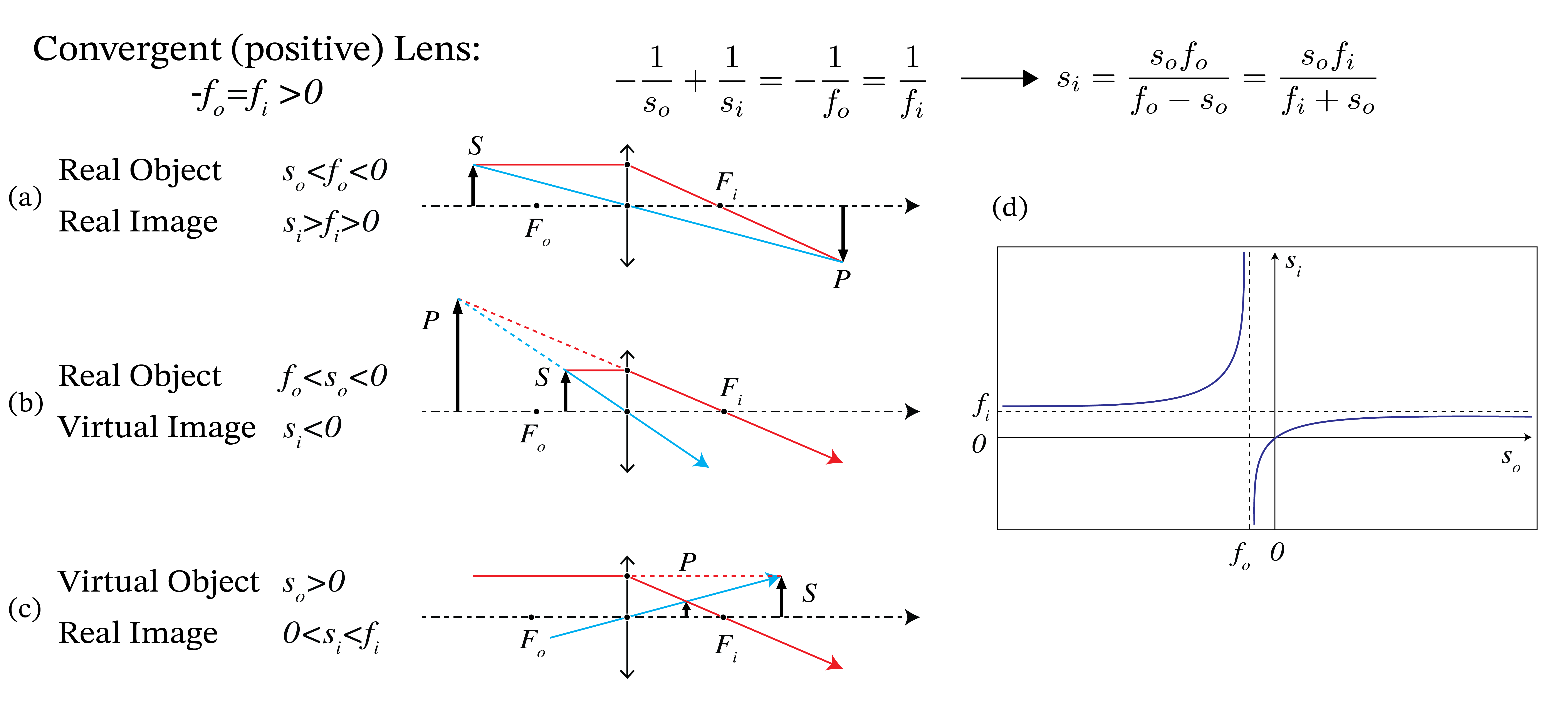
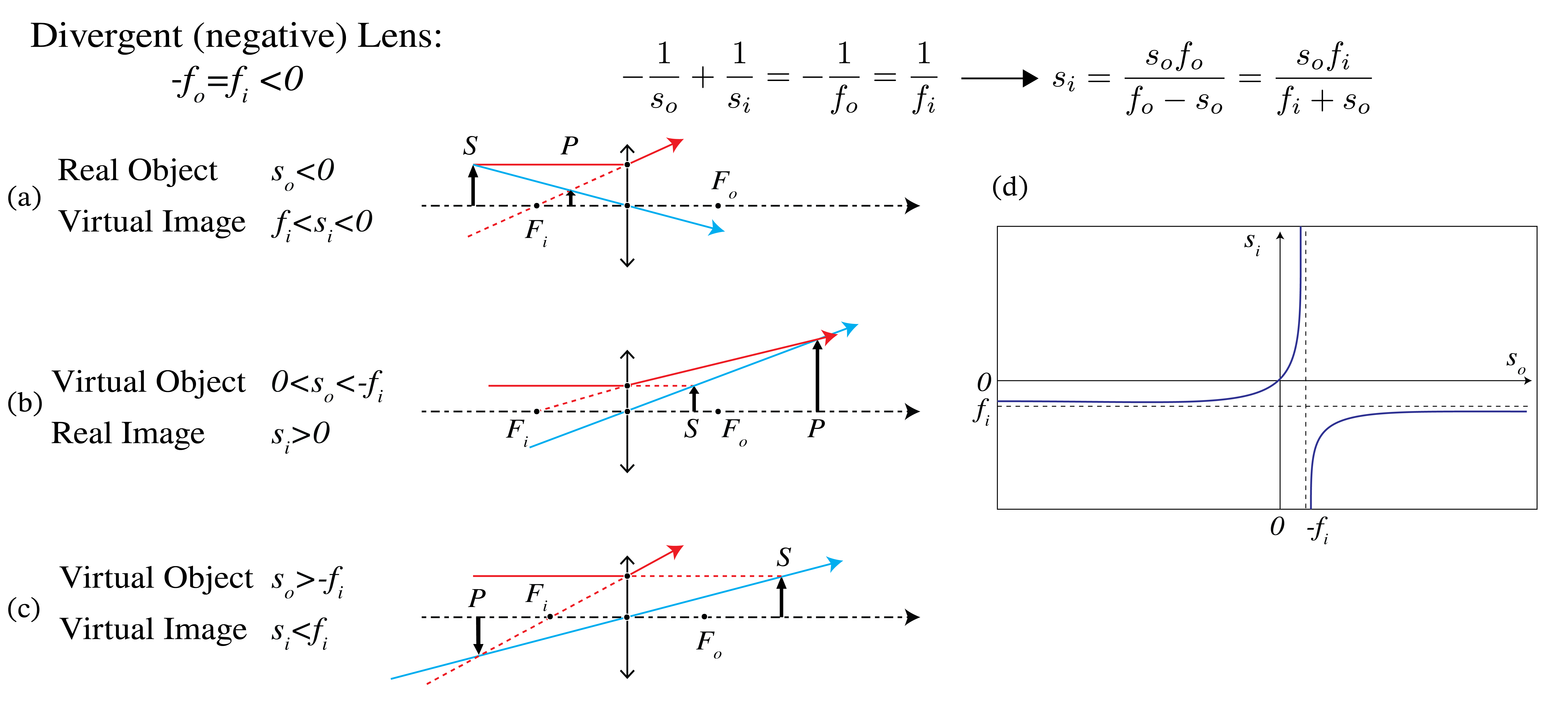
Examples of real and virtual object and image points for a positive and a negative lens are shown in Figure 6 and Figure 7.
Figure 6:Real and virtual objects and images for a convergent thin lens in the same medium on both sides, so −fo=fi>0. (a) A real object beyond the front focal point (so<fo) gives a real image (si>0). (b) A real object between that focal point and the lens (fo<so<0) gives a virtual image (si<0). (c) Incident rays converging toward a point behind the lens define a virtual object (so>0) and give a real image. (d) The graph shows si versus so from the thin-lens imaging equation.
Figure 7:Real and virtual objects and images for a divergent thin lens in the same medium on both sides, so −fo=fi<0. (a) A real object (so<0) gives a virtual image (si<0). For a virtual object, incident rays would converge at S behind the lens if the lens were absent. (b) If 0<so<−fi, the image is real. (c) If so>−fi, the image is virtual. (d) The graph shows si versus so from the thin-lens imaging equation.
The ray matrix is a suitable method to study the imaging of a system consisting of several thin lenses. For two lenses however, the imaging can still easily be obtained by construction.
We simply construct the image obtained by the first lens as if the second lens were not present and use this image as a (possibly virtual) object for the second lens.
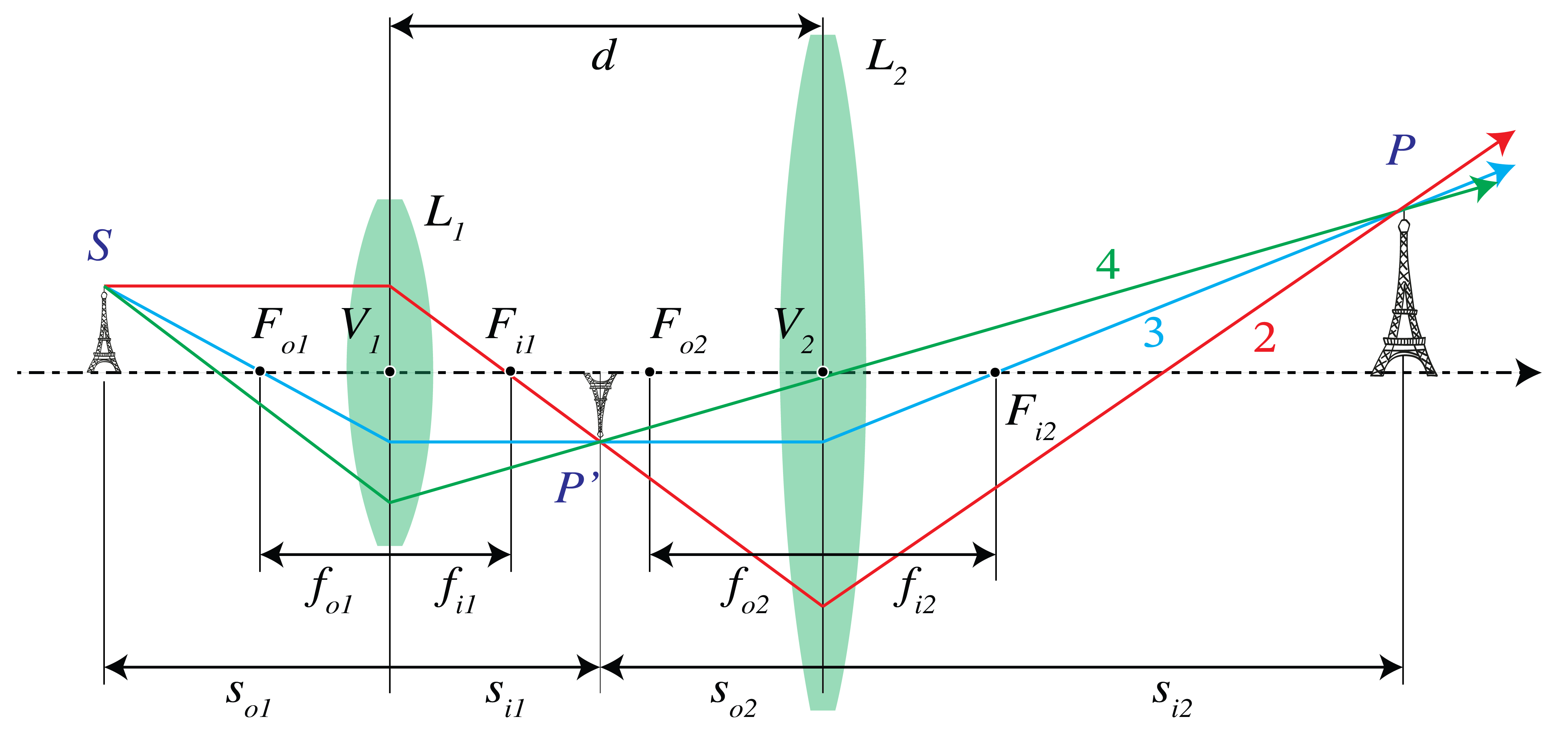
In Figure 8 an example is shown where the distance between the lenses is larger than the sum of their focal lengths.
First the image P′ of S is constructed as obtained by L1 as if L2 were not present.
We construct the intermediate image P′ due to lens L1 using rays 2 and 3. P′ is a real image for lens L1 and also a real object for lens L2. Ray 3 is parallel to the optical axis between the two lenses and is thus refracted by lens L2 through its back focal point F2i. Ray 4 is the ray from P′ through the center of lens L2. The image point P is the intersection of rays 3 and 4.
Figure 8:Two thin lenses separated by a distance that is larger than the sum of their focal lengths.
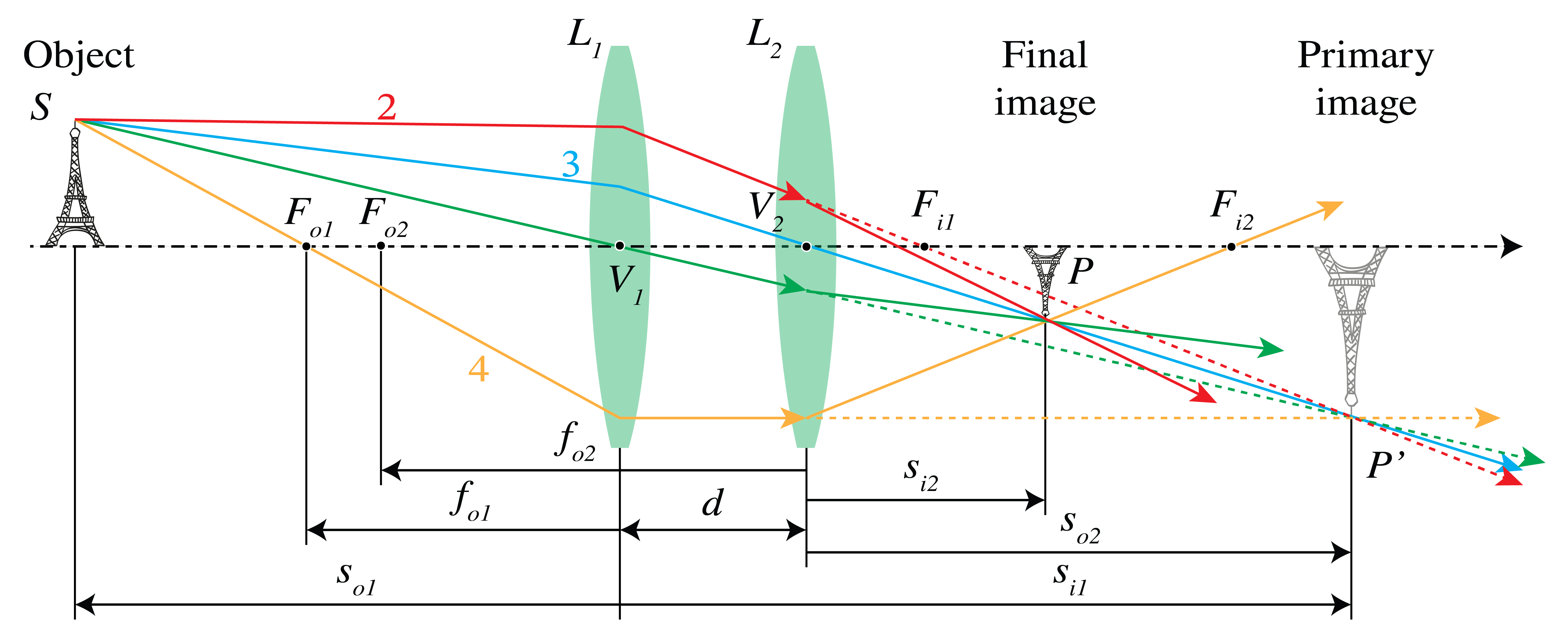
In the case of Figure 9 the distance d between the two positive lenses is smaller than their focal lengths.
The intermediate image P′ is a real image for L1 obtained as the intersection of rays 2 and 4 passing through the object and image focal points Fo1 and Fi1 of lens L1. P′ is now a virtual object for lens L2. To find its image by L2, draw ray 3 from P′ through the center of lens L2 back to S (this ray is refracted by lens L1 but not by L2) and draw ray 4 as refracted by lens L2. Since ray 4 is parallel to the optical axis between the lenses, it passes through the back focal point F2i of lens L2. The intersection point of rays 3 and 4 is the final image point P.
Figure 9:Two thin lenses at a distance smaller than their focal lengths.
It is easy to express the z-coordinate si with respect to the coordinate system with origin at the vertex V2 of the final image point, in terms of the z-coordinate so with respect to the origin at the vertex of lens L1 of the object point. We use the thin-lens imaging equation for each lens while taking care that the proper local coordinate systems are used.
The intermediate image P′ due to lens L1 has z-coordinate s1i with respect to the coordinate system with origin at the vertex V1, which satisfies:
As object for lens L2, P′ has z-coordinate with respect to the coordinate system with origin at V2 given by:
s2o=s1i−d, where d is the distance between the lenses. Hence, with si=s2i the imaging equation for lens L2 implies:
By taking the limit so→−∞, we obtain the z-coordinate fi of the image focal point of the two lenses, while si→∞ gives the z-coordinate fo of the object focal point:
We found in Section 2 that when the refractive indices of the
media before and after the lens are the same, the signed object and image focal
coordinates of a thin lens have equal magnitudes and opposite signs. As
Eq. (45) and Eq. (46) show, their
distances from the first and last vertices can differ for separated lenses.
By construction using the intermediate image, it is clear that the magnification of the two-lens system is the product of the magnifications of the two lenses:
In particular, by using two identical lenses in contact, the focal length is halved.
Although for two lenses the image coordinate can still be expressed
relatively easily in the object distance, for systems with more lenses
finding the overall ray matrix and then using the image condition Eq. (32) is a much better strategy.
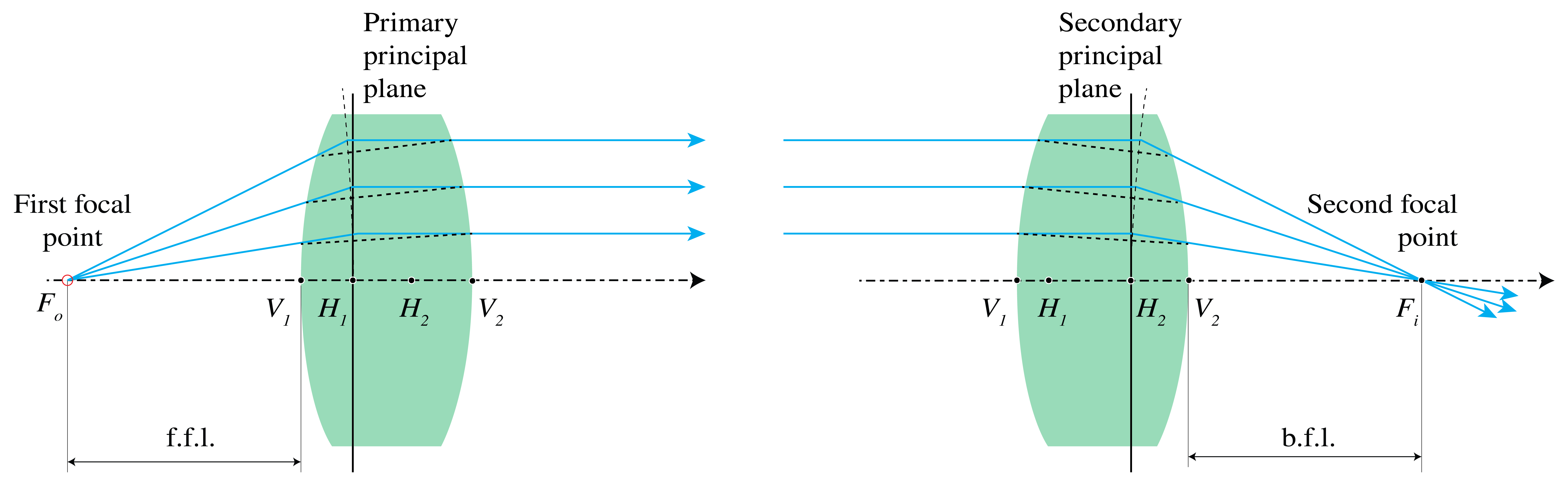
At the left of Figure 10 a thick lens is shown. The object focal point is defined as the point whose rays are refracted such that the emerging rays are parallel to the optical axis. By extending the incident and emerging rays by straight segments, the points of intersection are found to be on a curved surface which, close to the optical axis (in the paraxial approximation), is approximately a plane perpendicular to the optical axis. This plane is called the primary principal plane and its intersection with the optical axis is called the primary principal point H1.
Figure 10:Principal planes of a thick lens, with front and back focal lengths: f.f.l and b.f.l.
By considering incident rays which are parallel to the optical axis and therefore focused in the image focal point, the secondary principal plane and secondary principal point H2 are defined in a similar way (see the drawing at the right in Figure 10).
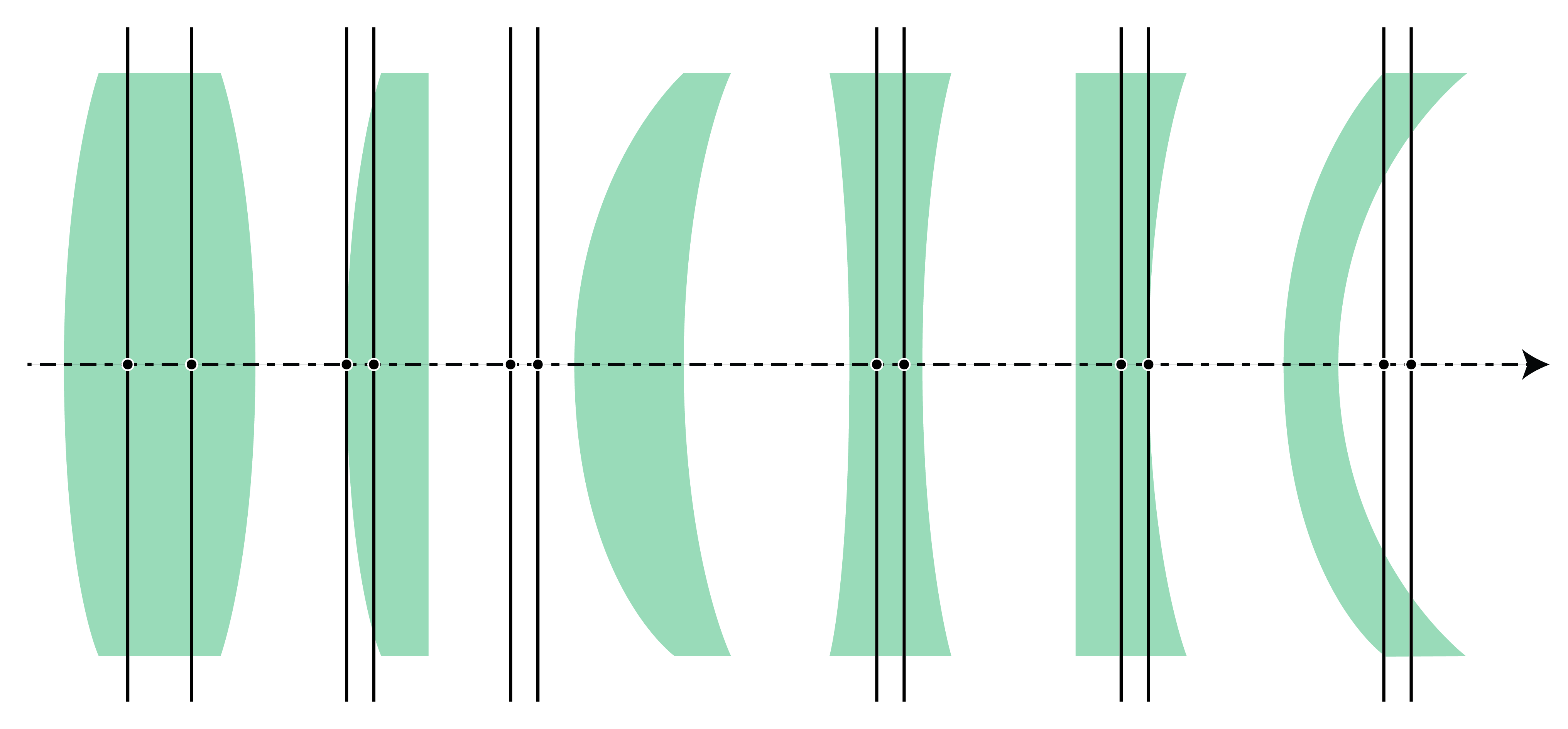
The principal planes can be outside the lens. For meniscus lenses, this is usually the case as shown in Figure 11.
It can be seen from Figure 10
that the principal planes are images of each other, with unit magnification. Hence, if an object is placed in the primary principal plane (hypothetically if this plane is inside the lens), its image is in the secondary principal plane. The image is erect and has unit magnification.
Figure 11:Position of the principal planes for several lenses.
Now, if the object coordinates and object focal point are defined with respect
to the origin at H1 and the image coordinates and image focal point are
defined with respect to the origin at H2, the imaging equation
Eq. (35) can also be used for a thick lens.
Proof
We recall the result Eq. (23) for the ray matrix between
the planes through the front and back vertices V1, V2 of a thick lens with
refractive index nl and thickness d:
If h1 is the z-coordinate of the first principal point H1 with respect
to the coordinate system with origin at vertex V1, we have according to Eq. (16) for the ray matrix between the primary
principal plane and the plane through vertex V1
Similarly, if h2 is the coordinate of the secondary principal point H2 with respect to the coordinate system with V2 as origin, the ray matrix between the plane through vertex V2 and the secondary principal plane is
The coordinates h1 and h2 can be found by imposing the imaging condition on the resulting matrix
Eq. (32): C=0 and the condition that the magnification
should be unity: D=1, which follows from Eq. (33).
We omit the details and only give the resulting expressions here:
We see that the ray matrix between the principal planes is identical to the
ray matrix of a thin lensEq. (25).
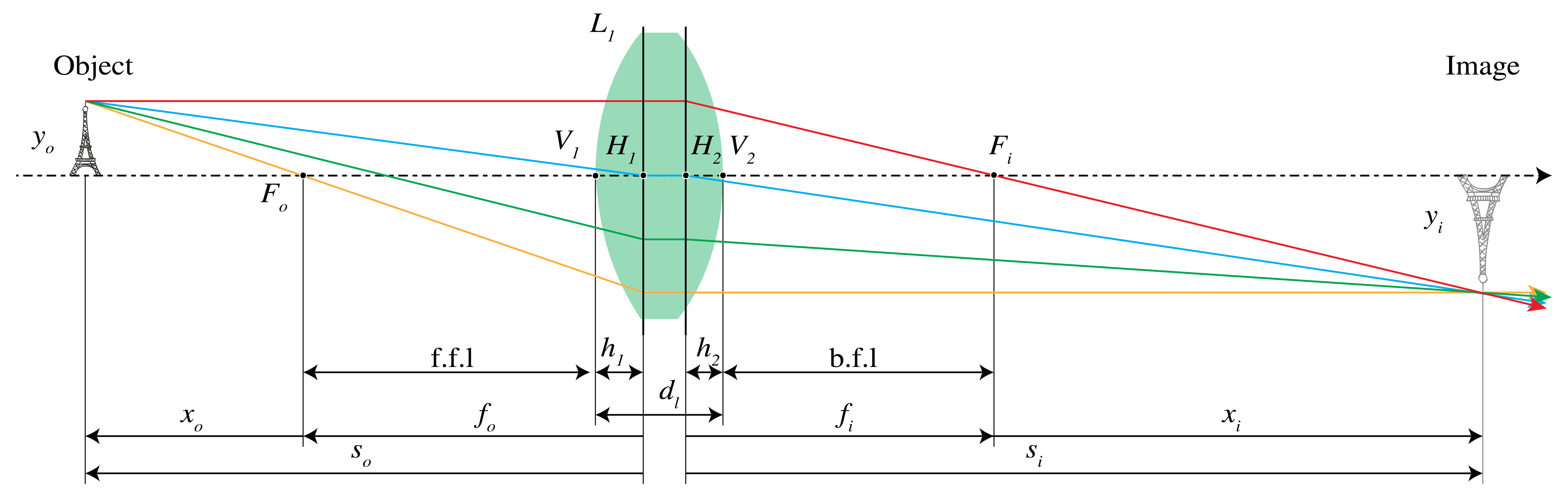
We therefore conclude that if the coordinates in object space are chosen with respect to the origin in the primary principal point H1, and the coordinates in image space are chosen with respect to the origin in the secondary principal point H2, the expressions for the first and second focal points and for the coordinates of the image point in terms of those of the object point are identical to those for a thin lens. An example of imaging by a thick lens is shown in Figure 12.
Figure 12:Thick-lens ray construction through the principal planes H1 and H2. When the external media have the same refractive index, the signed focal coordinates obey fi=−fo; object and image coordinates are measured from H1 and H2, respectively.
Ray vectors(nα,y)T describe a ray by its angle with the axis (weighted by refractive index) and its height.
Ray matrices (ABCD matrices) relate ray vectors before and after optical elements: (n2α2y2)=(ACBD)(n1α1y1).
System matrix: For multiple elements, multiply matrices in reverse order of light propagation.
Propagation matrix: (1d/n01) for distance d in medium with index n.
Spherical surface matrix: Power P=(n2−n1)/R; matrix has −P in upper right.
Thin lens matrix: (10−P1); its signed focal coordinates are fi=n2/P and fo=−n1/P.
Imaging condition: C=0 means two planes are conjugate (image each other).
Lensmaker formula: The thin-lens power follows from its surface curvatures; the imaging equation−n1/so+n2/si=P relates object and image coordinates.
Magnification: M=D when C=0; for equal external indices, Newton’s equation is xoxi=fofi=−fi2.
Two-lens systems: In air, the effective power is Peff=P1+P2−dP1P2; focal coordinates measured from the first and last lenses also depend on d.
Principal planes for thick lenses: The ray matrix between principal planes equals that of a thin lens.