1Polarization States and Jones Vectors
We have seen in Nature of Light that light is an electromagnetic wave which satisfies Maxwell’s equations and the wave equation derived therefrom. Since the electric field is a vector which oscillates as a function of time in a certain direction, we say that the wave has a certain polarization. In this chapter we look at the different types of polarization and how the polarization of a light beam can be manipulated.
From Maxwell’s equations and the wave equation, we know that the (real) electric field of a time-harmonic plane wave is always perpendicular to the direction of propagation, which is the direction of the wave vector as well as the direction of the Poynting vector (the direction of the power flow). Let the wave propagate in the -direction:
Then the electric field vector does not have a -component and hence the real electric field at and at time can be written as
where and are positive amplitudes and , are the phases of the electric field components. While and are fixed, we can vary , , and . This degree of freedom is why different states of polarization exist: the state of polarization is determined by the ratio of the amplitudes and by the phase difference between the two orthogonal components of the light wave Fowles, 1989. Consider the electric field in a fixed plane :
The complex vector
is called the Jones vector. It is used to characterize the polarization state. Let us see how, at a fixed position in space, the electric field vector behaves as a function of time for different choices of , and .
a) Linear polarization: or . When we have
Equality of the phases, , means that the field components and are in phase: when is large, is large, and when is small, is small. We can write
which shows that for the electric field simply oscillates in one direction given by the real vector . See Figure 1.
If we have
In this case and are out of phase and the electric field oscillates in the direction given by the real vector .
b) Circular polarization: , . In this case the Jones vector is:
The field components and are radians (90 degrees) out of phase: when is large, is small, and when is small, is large. We can write for and with :
At a given position, the electric field vector moves along a circle as time proceeds. For an observer looking towards the source, when the electric field rotates counterclockwise, we call it left-circularly polarized (+ sign in Eq. (9)); clockwise rotation is right-circularly polarized (- sign). This states the viewing direction explicitly because handedness names depend on convention.
c) Elliptical polarization: , and arbitrary. The Jones vector is:
In this case we get instead of Eq. (9) (again taking ):
This shows that the electric vector moves along an ellipse with major and minor axes parallel to the - and -axes. When the + sign applies, the field is called left-elliptically polarized, otherwise it is called right-elliptically polarized.
d) Elliptical polarization: anything else, and arbitrary. The Jones vector is now the most general one:
It can be shown that the electric field vector always moves along an ellipse. The exact shape and orientation of this ellipse vary with the difference in phase and the ratio of the amplitudes and and, except when , the major and minor axes of the ellipse are not parallel to the - and -axis. See Figure 3.
Remarks.
Frequently the Jones vector is normalized such that
The normalized vector represents of course the same polarization state as the unnormalized one. In general, multiplying the Jones vector by a complex number does not change the polarization state. If we multiply for example by , this has the same result as changing the instant at which , hence it does not change the polarization state. In fact:
A general time-harmonic field may superpose plane waves traveling in different directions, as near the focus of a high-numerical-aperture lens. There need not be one propagation direction perpendicular to the total electric field. At any fixed point, however, a harmonic real field has the form and traces an ellipse in the plane spanned by and ; a line and a circle are special cases. The plane may vary with position Born & Wolf, 1999. The Jones-vector treatment below applies to a single plane wave with a fixed transverse basis.

Figure 1:Linear polarization state of electromagnetic waves. The electric field vector oscillates along a single fixed direction perpendicular to the direction of propagation, tracing out a straight line in the plane perpendicular to the wave vector.

Figure 2:Circular polarization

Figure 3:Elliptical polarization
Illustration of different types of polarization. The horizontal and vertical arrows indicate the momentary field components . The thick arrow indicates the vector . The black curve indicates the trajectory of .
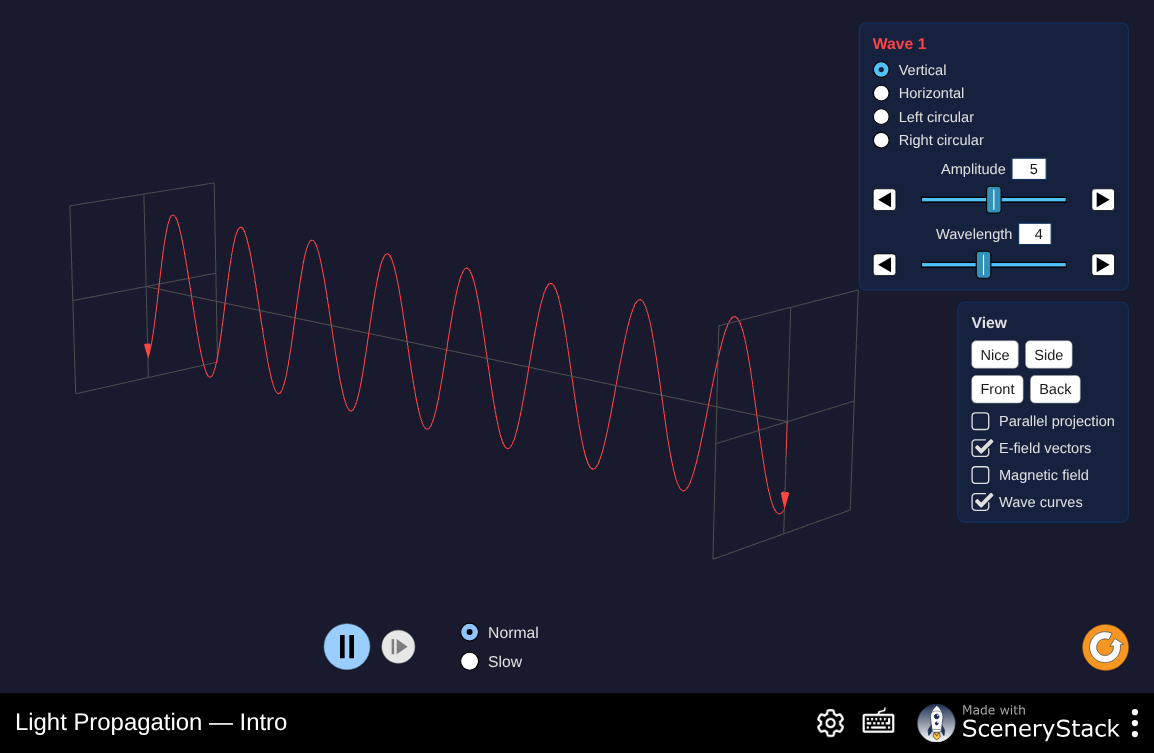
Figure 4:A monochromatic electromagnetic wave with its electric field drawn perpendicular to the propagation direction. Later screens of this simulation send the same wave through polarizers and birefringent plates — the interactive counterpart of the Jones-matrix section that follows.
Interactive simulation: Light Propagation
2Creating and Manipulating Polarization States
We have seen how Maxwell’s equations allow the existence of plane waves with many different states of polarization. But how can we create these states, and how do these states manifest themselves?
Natural light often does not have a definite polarization. Instead, the polarization fluctuates rapidly with time. To turn such randomly polarized light into linearly polarized light in a certain direction, we must extinguish the light polarized in the perpendicular direction. The remaining light is then linearly polarized along the desired direction. One could do this by using light reflected at the Brewster angle (which extinguishes p-polarized light), or one could let light pass through a dichroic crystal, which is a material which absorbs light polarized perpendicular to its so-called optic axis. A third method is sending the light through a wire grid polarizer, which consists of a metallic grating with sub-wavelength slits. Such a grating only transmits the electric field component that is perpendicular to the slits.
So suppose that with one of these methods we have obtained linearly polarized light. Then the question arises: how can linearly polarized light be changed into circularly or elliptically polarized light? Or how the state of linear polarization can be rotated over a certain angle? We have seen that the polarization state depends on the ratio of the amplitudes and on the phase difference of the orthogonal components and of the electric field. Thus, to change linearly polarized light to some other state of polarization, a certain phase shift (say ) must be introduced to one component (say ), and another phase shift to the orthogonal component . We can achieve this with a birefringent crystal, such as calcite. What is special about such a crystal is that it has two refractive indices: light polarized in a certain direction experiences a refractive index , while light polarized perpendicular to it feels another refractive index (the subscripts and stand for “ordinary” and “extraordinary”, but for our purpose we do not need to understand this terminology). The direction for which the refractive index is smallest (which can be either or ) is called the fast axis because its phase velocity is largest, and the other direction is the slow axis. Because there are two different refractive indices, one can see double images through a birefringent crystalHorvath et al., 2011. The difference between the two refractive indices is called the birefringence.
Suppose and that the fast axis, which corresponds to , is aligned with , while the slow axis (which then has refractive index ) is aligned with . If the wave travels a distance through the crystal, will accumulate a phase , and will accumulate , where is the vacuum wavelength. Thus, the phase difference increases by
2.1Jones Matrices
By letting light pass through crystals of different thicknesses we can create different phase differences between the orthogonal field components and in this way we can create different states of polarization. To be specific, let , as given by Eq. (4), be the Jones vector of the plane wave before the crystal. Then we have, for the Jones vector after the passage through the crystal:
where
A matrix such as , which transfers one state of polarization of a plane wave into another, is called a Jones matrix. Depending on the phase difference which a wave accumulates by traveling through the crystal, these devices are called quarter-wave plates (phase difference ), half-wave plates (phase difference ), or full-wave plates (phase difference ). The applications of these wave plates will be discussed in later sections.
Consider as an example the Jones matrix which describes the change of linearly polarized light into circular polarization. Assume that we have diagonally (linearly) polarized light, so that
We want to change it to circularly polarized light, for which
where one can check that indeed . This can be done by passing the light through a crystal such that accumulates a phase difference of with respect to . The transformation by which this is accomplished can be written as
The matrix on the left is the Jones matrix describing the operation of a quarter-wave plate.
Another important Jones matrix is the rotation matrix. In the preceding discussion it was assumed that the fast and slow axes were aligned with the - and -direction (i.e. they were parallel to and ). Suppose now that the slow and fast axes of the wave plate no longer coincide with and , but rather with some other and as in Figure 5. In that case we apply a basis transformation: the electric field vector which is expressed in the , basis should first be expressed in the , basis before applying the Jones matrix of the wave plate to it. After applying the Jones matrix, the electric field has to be transformed back from the , basis to the , basis.
Let be given in terms of its components on the , basis:
To find the components , on the , basis:
We first write the unit vectors and in terms of the basis , (see Figure 5)
By substituting Eq. (23) and Eq. (24) into Eq. (22) we find
Comparing with Eq. (21) implies
where is the rotation matrix over an angle in the counterclockwise direction: Hecht, 2002.
That indeed is a rotation through an angle in the counterclockwise direction is easy to see by considering what happens when is applied to the vector Hecht, 2002.
This relationship converts Jones-vector components from the crystal’s axes to the original axes. The reverse conversion is . If is the wave-plate matrix in Eq. (17), with as the fast axis and as the slow axis, then the matrix of the rotated plate in the , basis is
This is a standard result from linear algebra involving basis transformations.
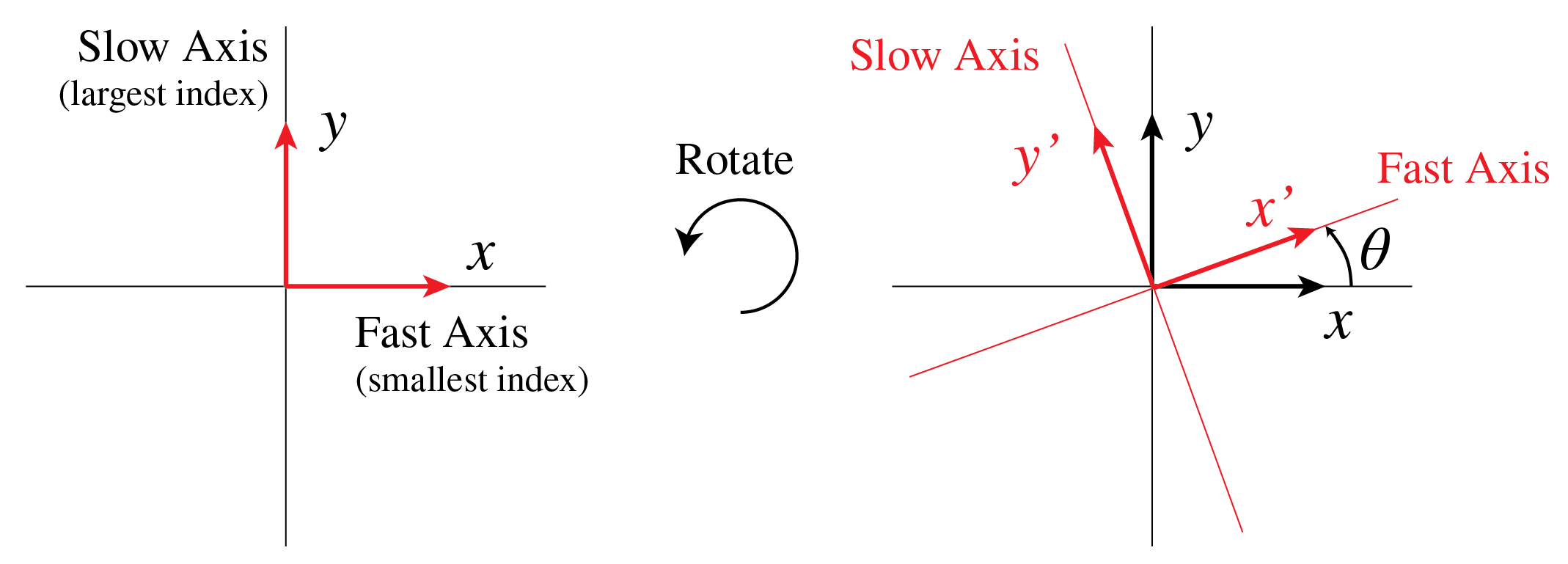
Figure 5:If the wave plate is rotated, the fast and slow axes no longer correspond to and . Instead, we have to introduce a new coordinate system ().
2.2Linear polarizers
A polarizer that only transmits horizontally polarized light is described by the Jones matrix:
Clearly, horizontally polarized light is completely transmitted, while vertically polarized light is not transmitted at all. More generally, for light that is polarized at an angle , we get
The amplitude of the transmitted field is reduced by the factor , which implies that the intensity of the transmitted light is reduced by the factor . This relation is known as Malus’ law.
2.3Degree of Polarization
Natural light such as sunlight is unpolarized. The instantaneous polarization of unpolarized light fluctuates rapidly in a random manner. A linear polarizer produces linearly polarized light from unpolarized light. It follows from Eq. (29) that the intensity transmitted by a linear polarizer when unpolarized light is incident is the average value of namely , times the incident intensity.
Light that is a mixture of polarized and unpolarized light is called partially polarized. The degree of polarization is defined as the fraction of the total intensity that is polarized:
2.4Quarter-Wave Plates
Figure 6:A birefringent slab with adjustable retardation. Set a quarter-wave or half-wave plate, rotate the fast axis relative to a linear input, and watch linear light become circular (or rotate) — the same phase shift treated by the Jones matrix below.
Interactive simulation: Light Propagation
A quarter-wave plate has already been introduced above. It introduces a phase shift of , so its Jones matrix is
because . To describe the actual transmission through the quarter-wave plate, the matrix should be multiplied by some global phase factor, but because we only care about the phase difference between the field components, this global phase factor can be omitted without problem. The quarter-wave plate is typically used to convert linearly polarized light to elliptically polarized light and vice-versaSaleh & Teich, 2007. If the incident light is linearly polarized at angle , the state of polarization after the quarter-wave plate is
In particular, if incident linear polarization is at to either plate axis, the output is circularly polarized. Conversely, circular input becomes linearly polarized after an ideal quarter-wave plate.
A demonstration is shown inBartholinus, 1669.
2.5Half-Wave Plates
A half-wave plate introduces a phase shift of , so its Jones matrix is
because . An important application of the half-wave plate is to change the orientation of linearly polarized lightFowles, 1989. After all, what this matrix does is mirror the polarization state in the -axis. Thus, if we choose our mirroring axis correctly (i.e. if we choose the orientation of the wave plate correctly), we can change the direction in which the light is linearly polarized arbitrarilyGoldstein, 2011. To give an example: a wave with linear polarization parallel to the -direction can be rotated by an angle by rotating the crystal such that the fast axis makes an angle with the -axis. Upon propagation through the crystal, the slow axis gets an additional phase of , due to which the electric vector makes angle with the -axis (see Figure 5). It is not difficult to verify that when the fast and slow axes are interchanged, the same linear state of polarization results.
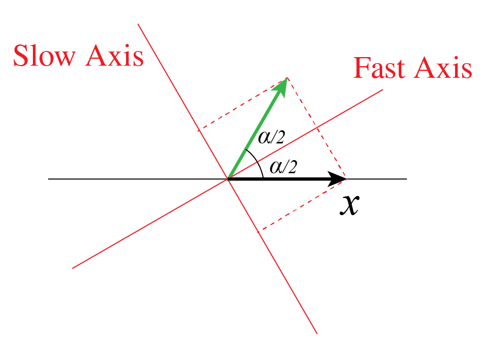
Figure 7:Rotation of horizontally polarized light by an angle using a half-wave plate.
2.6Full-Wave Plates
A full-wave plate introduces a phase difference of , which is the same as introducing no phase difference between the two field components. So what can possibly be an application for a full-wave plate? We recall from Eq. (15) that the phase difference is only for a particular wavelength. To obtain wavelength-dependent transmission, orient the incident linear polarization at to the plate’s axes and place a crossed analyzer after the plate. At the design wavelength , the full-wave plate restores the incident polarization and the analyzer extinguishes it. Nearby wavelengths acquire a different relative phase and can pass partially. Other wavelengths with integer-wave retardance are also extinguished, so this arrangement does not select a unique wavelength.
3More on Jones matrices
If the direction of either the slow or fast axis and the ordinary and extra-ordinary refractive indices and are given, it is easy to write down the Jones matrix of a birefringent plate of given thickness using the rotation matrices, see Eq. (27). Instead of using the rotation matrices, one can also write down a system of equations for the elements of the Jones matrix. Suppose that and are in the direction of the ordinary and the extra-ordinary axes, respectively. Then if the Jones matrix is
then
where . Equating components implies
Similarly, for a linear polarizer it is simple to write down the Jones matrix if one knows the direction in which the polarizer absorbs or transmits all the light: use Eq. (28) in combination with the rotation matrices. Alternatively, if is in the direction of the linear polarizer and is perpendicular to it, we have
which is a system of equations of type Eq. (37) for the elements of the Jones matrix.
Suppose now that the complex (2,2)-matrix Eq. (35) is given. How can one verify whether this matrix corresponds to a linear polarizer or to a wave plate? Note that the elements of a Jones matrix are in general complex.
1. Linear polarizer. An ideal lossless linear polarizer transmits one real linear-polarization direction and blocks its orthogonal direction. Up to an overall phase, its eigenvalues are 1 and 0, with orthogonal eigenvectors that can be chosen real. A Jones matrix with eigenvalues 2 and 0 would amplify the transmitted field, so it is not a passive ideal polarizer. Eigenvectors that cannot be chosen real do not identify two linear-polarization directions.
2. Wave plate. To show that the matrix corresponds to a wave plate, there should exist two real orthogonal eigenvectors with, in general, complex eigenvalues of modulus 1. In fact, one of the eigenvectors corresponds to the ordinary axis with refractive index , and the other to the extra-ordinary axis with refractive index . The eigenvalues are then
where is the plate thickness and is the vacuum wave number. Thus, a lossless linear wave plate has two orthogonal real eigenvectors and eigenvalues of unit modulus. A global phase factor does not affect its polarization action.
3. Jones matrix for propagation through sugars. In sugars, left and right circularly polarized light propagate with their own refractive index. Therefore sugars are called circularly birefringent. The matrix Eq. (35) corresponds to propagation through sugar when there are two real orthogonal unit vectors and such that the circular polarization states
are eigenstates of with complex eigenvalues with modulus 1.
4Decomposition of an Elliptical Polarization State into Linear and Circular States
Any elliptical polarization state can be written as the sum of two perpendicular linearly polarized states:
Furthermore, any elliptical polarization state can be written as the sum of two circular polarization states, one right-circularly polarized and the other left-circularly polarized:
We conclude that to study what happens to elliptic polarization, it suffices to consider two orthogonal linear polarizations, or, if that is more convenient, left- and right-circular polarized light. In a birefringent material each of the two linear polarizations, namely parallel to the o-axis and parallel to the e-axis, propagates with its own refractive index. To predict what happens to an arbitrary linear polarization state which is not aligned to either of these axes, or more generally what happens to an elliptical polarization state, we write this polarization state as a linear combination of o- and e-states, i.e. we expand the field on the o- and e-basis.
To see what happens to an arbitrary elliptical polarization state in a circular birefringent material, the incident light is best written as a linear combination of left and right circular polarizations.
5Chapter Summary
Polarization describes the orientation of the electric field vector oscillation in an electromagnetic wave.
Linear polarization: The electric field oscillates in a fixed direction; described by a Jones vector with real components.
Circular polarization: The electric field rotates at constant amplitude; left-circular and right-circular have opposite handedness.
Elliptical polarization: The most general fully polarized state; the electric field traces an ellipse set by component amplitudes and relative phase.
Jones vectors represent polarization states as 2D complex vectors; Jones matrices describe how optical elements transform polarization.
Polarizers transmit one polarization and block the orthogonal one; Malus’s Law gives transmitted intensity as .
Birefringence occurs when a material has different refractive indices for different polarization directions.
Wave plates: Quarter-wave plates convert linear to circular polarization (and vice versa); half-wave plates rotate linear polarization.
Circular birefringence gives the two circular components different phase shifts and can rotate linear polarization.
Degree of polarization measures the polarized fraction of a beam’s total intensity.
6References
- Fowles, G. R. (1989). Introduction to Modern Optics. Dover Publications.
- Born, M., & Wolf, E. (1999). Principles of Optics (7th ed.). Cambridge University Press.
- Horvath, G., Barta, A., Pomozi, I., Suhai, B., Hegedus, R., Åkesson, S., Meyer-Rochow, B., & Wehner, R. (2011). Viking navigation using polarized skylight. Proceedings of the Royal Society A: Mathematical, Physical and Engineering Sciences, 467(2127), 651–660.
- Hecht, E. (2002). Optics (4th ed.). Addison Wesley.
- Saleh, B. E. A., & Teich, M. C. (2007). Fundamentals of Photonics (2nd ed.). Wiley-Interscience.
- Bartholinus, E. (1669). Experimenta crystalli islandici disdiaclastici quibus mira & insolita refractio detegitur. Copenhagen: Daniel Paulli.
- Fowles, G. R. (1989). Introduction to Modern Optics. Dover Publications.
- Goldstein, D. H. (2011). Polarized Light (3rd ed.). CRC Press.