In the early 1950s a new source of microwave radiation, the maser, was invented by C.H. Townes in the USA and A.M. Prokhorov and N.G. Basov in the USSR. Maser stands for “Microwave Amplification by Stimulated Emission of Radiation”. In 1958, A.L. Schawlow and Townes formulated the physical conditions for realizing a similar device for visible light. This resulted in 1960 in the first optical maser by T.H. Maiman in the USA. This device has since been called Light Amplification by Stimulated Emission of Radiation or laser. It has revolutionized science and engineering and has many applications, e.g.
bar code readers,
compact discs,
computer printers,
fiber optic communication,
sensors,
material processing,
non-destructive testing,
position and motion control,
medical applications, such as treatment of retina detachment,
nuclear fusion,
holography.
1Unique Properties of Lasers
The broad application of lasers is made possible by the unique properties that distinguish lasers from all other light sources. We discuss these unique properties below.
1.1Narrow Spectral Width; High Temporal Coherence
A narrow spectrum generally corresponds to a long temporal coherence time; the precise relationship depends on spectral shape. A spectral lamp, such as a mercury-vapor discharge lamp, can have a spectral width of GHz. At nm the optical frequency is about Hz, so the fractional width is about . The line width measured in wavelengths satisfies
For this example, nm. A laser with a 10 MHz linewidth is narrower by a factor of 1000; at 550 nm its wavelength width is about 10-5 nm. These are illustrative linewidths. As explained in Chapter 6, the coherence time is of the order of the reciprocal frequency bandwidth:
Light is emitted by atoms in bursts of harmonic (cosine) waves consisting of a great but finite number of periods. As will be explained in this chapter, due to the special configuration of the laser, the wave trains in laser light can be extremely long, corresponding to a very long coherence time.
1.2Highly Collimated Beam
Consider a discharge lamp as shown in Figure 1.
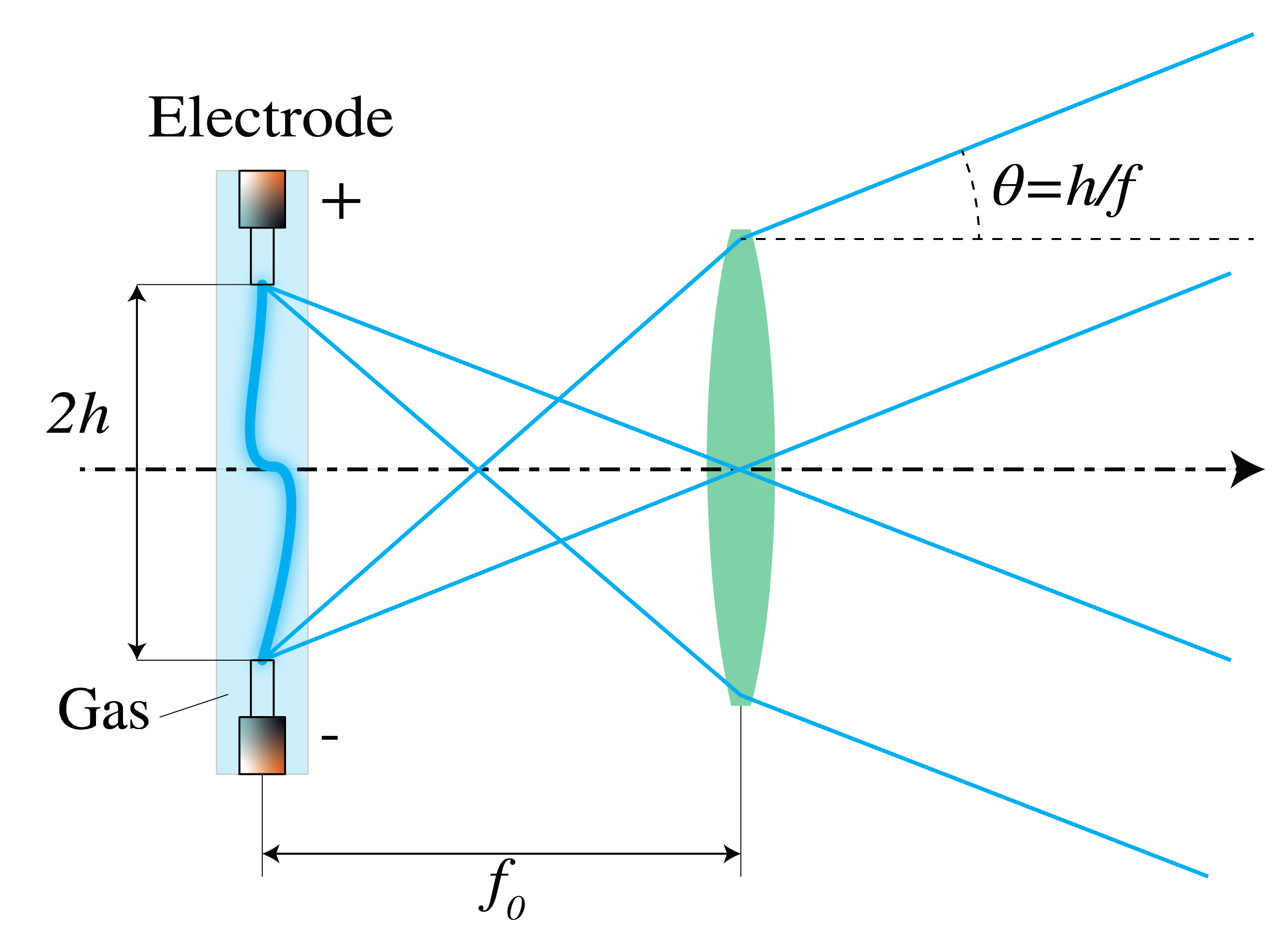
Figure 1:A discharge lamp in the focal plane of a converging lens. Every atom in the lamp emits a spherical wave during a burst of radiation, lasting on average a coherence time . The overall divergence of the beam is determined by the atoms at the extreme positions of the source.
To collimate the light, the lamp can be positioned in the focal plane of a lens. The spherical waves emitted by the atoms (point sources) in the lamp are collimated into plane waves whose direction depends on the position of the atoms in the source. The atoms at the edges of the source determine the overall divergence angle , which is given by
where is the size of the source and is the focal length of the lens as shown in Figure 1. Hence the light can be collimated by either choosing a lens with large focal length or by reducing the size of the source, or both. Both methods lead, however, to weak intensities. Due to the special configuration of the laser source, which consists of a Fabry-Perot resonator in which the light bounces up and down many times before being emitted, the atomic sources are effectively all at a very large distance and hence the effective size of the source is very small. The divergence of a well-designed single-transverse-mode laser is then governed mainly by diffraction at its output beam aperture. As follows from Scalar Diffraction Optics, the characteristic diffraction angle of a beam with diameter and wavelength scales as:
The diffraction-limited divergence thus depends on the wavelength and decreases when the diameter of the emitting surface increases. With a suitable single-mode laser, the diffraction-limited divergence angle can nearly be reached and therefore a collimated beam with very high intensity can be realized (Figure 2).
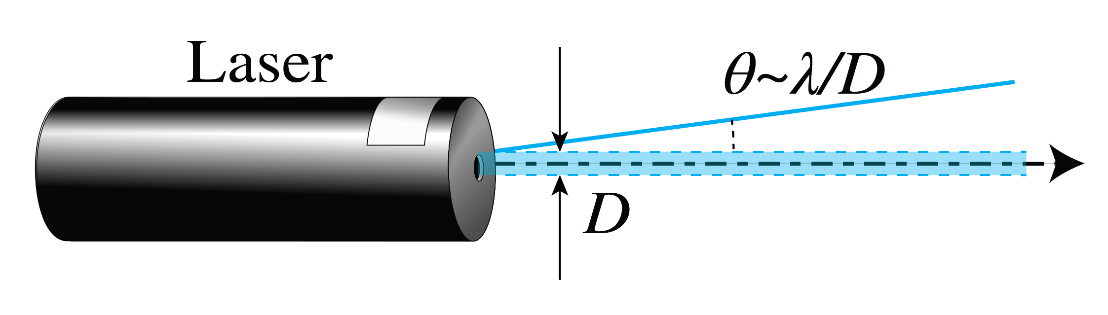
Figure 2:A laser beam can almost reach diffraction-limited collimation.
1.3Diffraction-Limited Focused Spot, High Spatial Coherence
For a uniformly filled circular lens aperture of diameter , focal length , and small-angle numerical aperture in air, the radius to the first dark Airy ring is, according to Scalar Diffraction Optics,
With a laser one can achieve a diffraction-limited spot with a very high intensity.
As has been explained in Interference and Coherence, a light wave has high spatial coherence if at any given time, its amplitude and phase at different points can be predicted. The spherical waves emitted by a point source have this property. But when there are many point sources (atoms) that each emit bursts of harmonic waves that start at random times, as is the case in a classical light source, the amplitude and phase of the total emitted field at any position in space cannot be predicted. The only way to make the light spatially coherent is by making the light source very small, but then there is hardly any light. As will be explained below, by the design of the laser, the emissions by the atoms of the amplifying medium in a laser are phase-correlated, which leads to a very high temporal and spatial coherence.
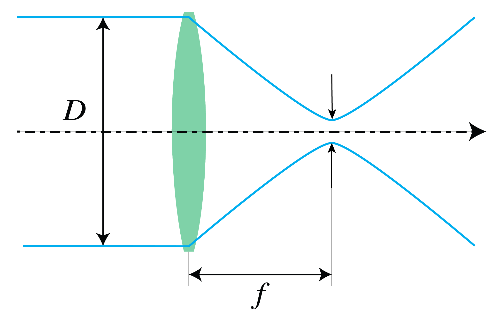
Figure 3:Diffraction-limited spot obtained by focusing a collimated beam.
A small, bright focal spot is useful in high-resolution imaging, material processing, and carefully controlled ophthalmic laser procedures.
1.4High Power
Lasers can operate in continuous-wave (CW) mode or emit pulses. These pulses can be very short: from nanoseconds to even femtoseconds (10-15 s). A relatively low-power CW laser is the HeNe laser which emits roughly 1 mW at the wavelength 632 nm. Some continuous-wave lasers deliver kilowatts of output power. Because their energy is delivered over a short duration, pulsed lasers can reach peak powers far above their average output power.
There are many applications of high-power lasers such as for cutting and welding materials. To obtain EUV light with sufficiently high intensity for use in photolithography for manufacturing ICs, extremely powerful CO lasers are used to excite a plasma. Extremely high-power lasers are also applied to initiate fusion and in many nonlinear optics applications. Lasers with very short pulses are used to study very fast phenomena with short decay times.
1.5Wide Tuning Range
For a wide range of wavelengths, from the vacuum ultra-violet (VUV), the ultra-violet (UV), the visible, the infrared (IR), the mid-infrared (MIR) up into the far infrared (FIR), lasers are available. For some types of lasers, the tuning range can be quite broad. The gaps in the electromagnetic spectrum that are not directly addressed by laser emission can be covered by techniques such as higher harmonic generation and frequency differencing.
2Optical Resonator
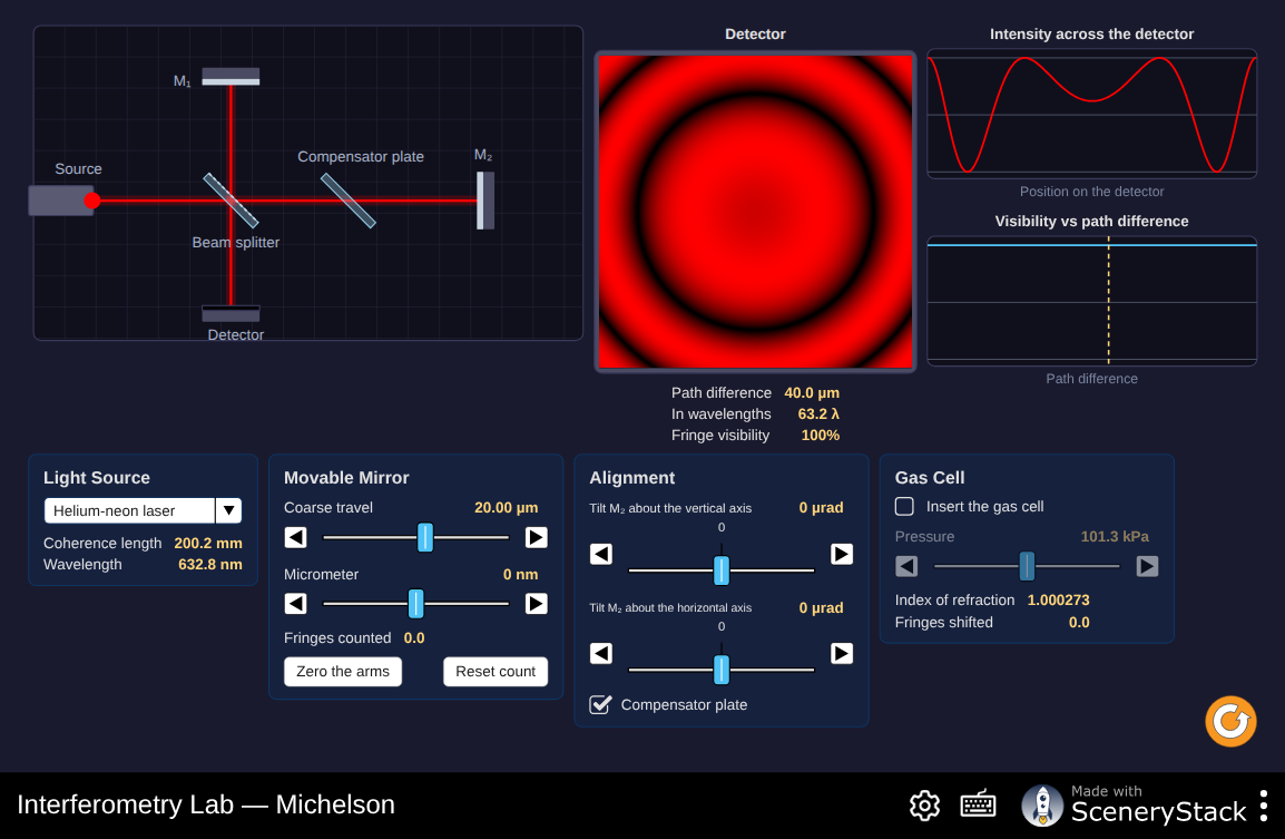
Figure 4:The same Fabry–Pérot geometry that appears as a spectrometer in Interference and Coherence, now read as a laser cavity: raise the mirror reflectance and watch the resonance peaks sharpen. The amplifying medium and population inversion are treated interactively in Figure 9.
Interactive simulation: Interferometry Lab
We now explain the working of lasers. A laser consists of
an optical resonator;
an amplifying medium.
In this section we consider the resonator. Its function is to obtain a high light energy density and to gain control over the emission wavelengths.
A mechanical or electrical resonator has one or more resonance frequencies . Without energy input, losses make its amplitude decay, as shown in Figure 5. The resulting spectrum has a finite width of order , where is a characteristic decay time. The numerical coefficient depends on how the linewidth and decay time are defined.
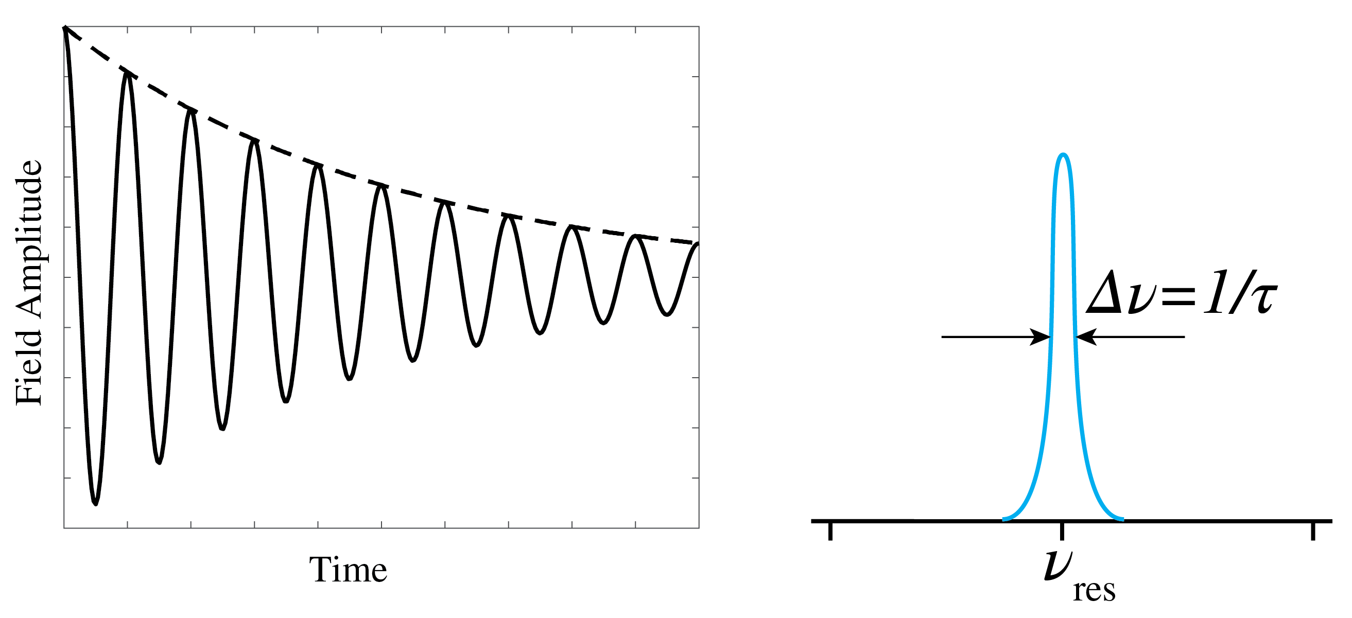
Figure 5:Damped field amplitude versus time (left) and its broadened resonance spectrum versus frequency (right); a shorter decay time gives a wider spectral line.
The optical resonator is a Fabry-Perot resonator filled with some material with refractive index bounded by two aligned, highly reflective mirrors at a distance . The Fabry-Perot resonator is discussed extensively in the Fabry-Perot Interferometer section of the Interference chapter but to understand this chapter a detailed analysis of the Fabry-Perot is not needed.
Let the -axis be chosen along the axis of the cavity as shown in Figure 6, and assume that the transverse directions are so large that the light can be considered a plane wave bouncing back and forth along the -axis between the two mirrors. Let be the frequency and the wave number in vacuum. The plane wave that propagates in the positive -direction is given by:
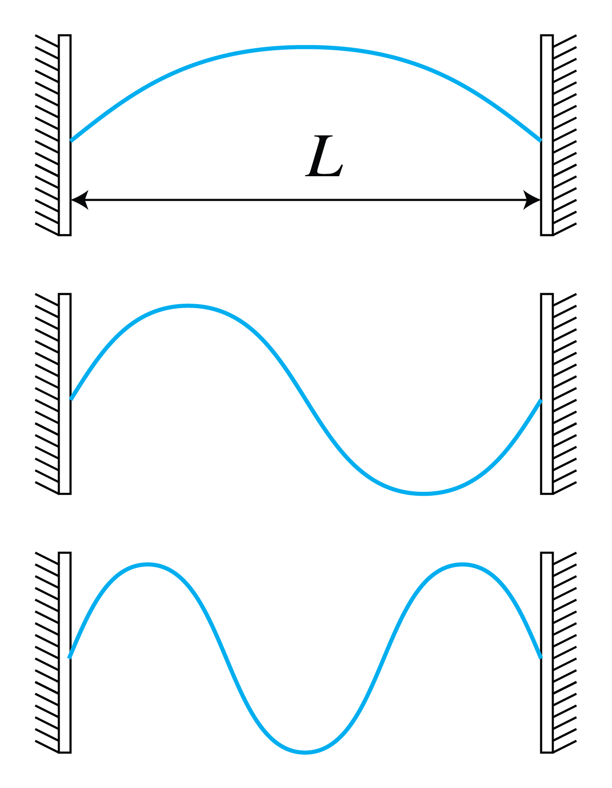
Figure 6:Fabry-Perot resonances.
For ideal mirrors that each contribute the same reflection phase, the two reflection phases add to an integer multiple of . Neglecting loss, the field after one round trip is:
A high field builds up when this wave constructively interferes with Eq. (6), i.e. when
for . Hence, provided dispersion of the medium can be neglected (i.e. is independent of the frequency), the resonance frequencies are separated by
which is the so-called free spectral range. For a gas laser of length 1 m, the free spectral range is approximately 150 MHz.
2.1Example: Cavity Mode Number
Suppose that the cavity is 100 cm long and is filled with a material with refractive index . Light with visible wavelength of nm corresponds to mode number and the free spectral range is MHz.
The multiple reflections of the laser light inside the resonator make the optical path length very large. For an observer, the atomic sources seem to be at a very large distance and the light that is exiting the cavity resembles a plane wave. As explained above, the divergence of the beam is therefore not limited by the size of the source, but by diffraction due to the aperture of the exit mirror.
Because of losses caused by the mirrors (which never reflect perfectly) and by the absorption and scattering of the light, the resonances have a certain frequency width . When a resonator is used as a laser, one of the mirrors is given a small transmission to couple the laser light out and this also contributes to the loss of the resonator. To compensate for all losses, the cavity must contain an amplifying medium. Due to the amplification, the resonance line widths inside the bandwidth of the amplifier are reduced to very sharp lines as shown in Figure 7.
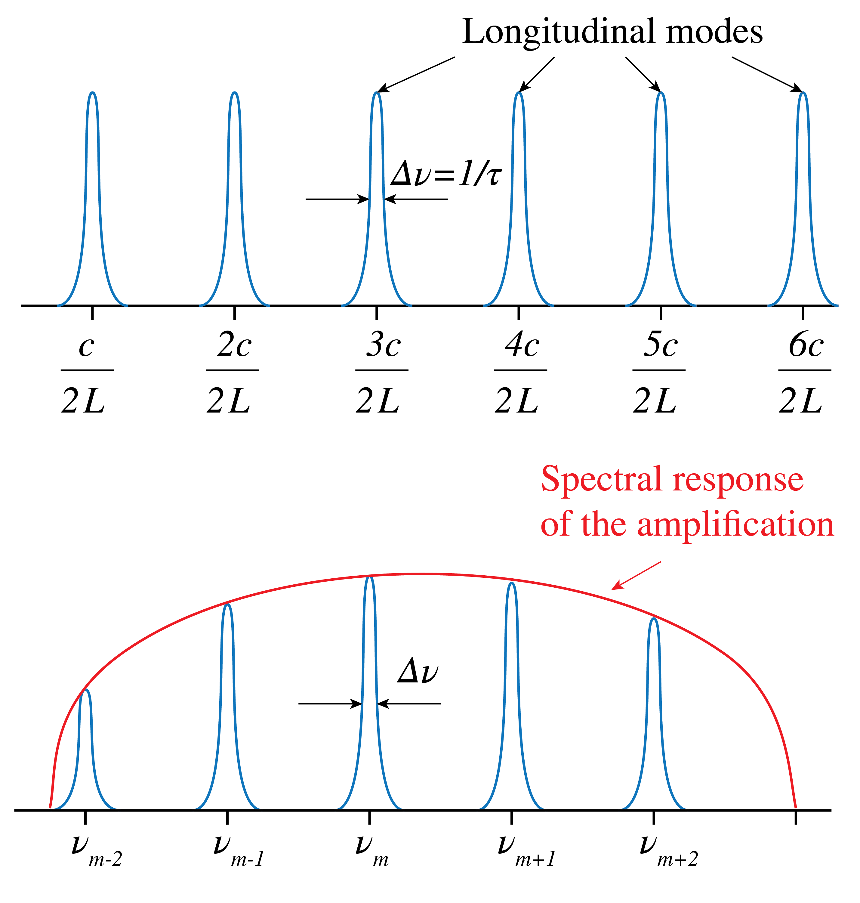
Figure 7:Resonant frequencies of a cavity of length when the refractive index . With an amplifier inside the cavity, the line widths of the resonances within the bandwidth of the amplifier are reduced. The envelope is the spectral function of the amplification.
3Amplification
Amplification can be achieved by a medium with atomic resonances that are at or close to one of the resonances of the resonator. We first recall the simple theory developed by Einstein in 1916 of the dynamic equilibrium of a material in the presence of electromagnetic radiation.
3.1The Einstein Coefficients
We consider two atomic energy levels . By absorbing a photon of energy
an atom that is initially in the lower energy state 1 can be excited to state 2. Here is the reduced Planck constant:
Suppose is the time-averaged electromagnetic energy density per unit of frequency interval around frequency . Hence has units . Let and be the number of atoms in states 1 and 2, respectively, where
is the total number of atoms (which is constant). The rate of absorption is the rate of decrease of and is proportional to the energy density and the number of atoms in state 1:
where the constant has dimension . Without any external influence, an atom that is in the excited state will usually transfer to state 1 after a lifetime that depends on the transition, while emitting a photon of energy Eq. (10). This process is called spontaneous emission, since it happens also without an electromagnetic field present. The rate of spontaneous emission is given by:
where has dimension . The lifetime of spontaneous emission is . It is important to note that the spontaneously emitted photon is emitted in a random direction. Furthermore, since the radiation occurs at a random time, there is no phase relation between the spontaneously emitted field and the field that excites the atom.
It is less obvious that in the presence of an electromagnetic field of frequency close to the atomic resonance, an atom in the excited state can also be stimulated by that field to emit a photon and transfer to the lower energy state. The rate of stimulated emission is proportional to the number of excited atoms and to the energy density of the field:
where has the same dimension as . It is very important to remark that stimulated emission occurs in the same electromagnetic mode (e.g. a plane wave) as the mode of the field that stimulates the transition and that the phase of the radiated field is identical to that of the exciting field. This implies that stimulated emission enhances the electromagnetic field by constructive interference. This property is crucial for the operation of the laser.
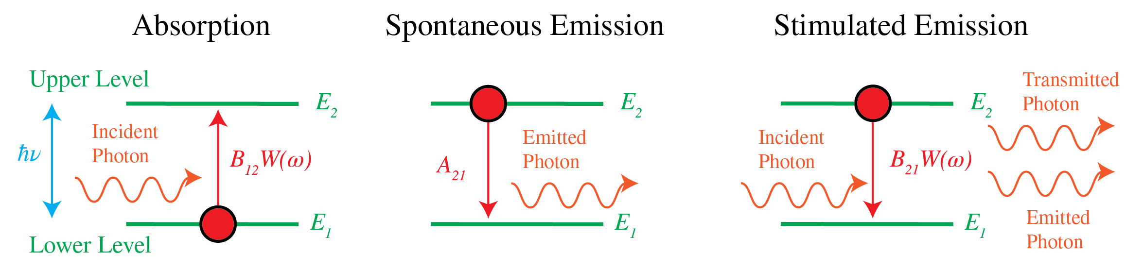
Figure 8:Absorption, spontaneous emission and stimulated emission.
3.2Relation Between the Einstein Coefficients
The Einstein coefficients , and are related. Here the two levels are assumed to have equal statistical weights; unequal degeneracies modify the relation between and . Consider a black body, such as a closed empty box. Because no radiation enters or leaves the box, after a certain time the electromagnetic energy density is the thermal density , which, according to Planck’s Law, is independent of the material of which the box is made and is given by:
where is Boltzmann’s constant:
The rates of upward and downward transitions of the atoms in the wall of the box must be identical:
Hence,
But in thermal equilibrium:
By substituting Eq. (20) into Eq. (19), and comparing the result with Eq. (16), it follows that both expressions for are identical for all temperatures only if
3.3Example: Einstein Coefficients Ratio
For green light of nm, and thus
Hence the spontaneous and stimulated emission rates are equal if .
For a (narrow) frequency band the time-averaged energy density is and for a plane wave the energy density is related to the intensity (i.e. the length of the time-averaged Poynting vector) by:
For an illustrative frequency interval of 1010 Hz, . The equal-rate spectral density above corresponds to an intensity of about concentrated in that interval. The representative intensities in Table 1 alone cannot determine the stimulated-emission rate: the spectral energy density at the transition frequency is what matters.
Table 1:Typical intensities of light sources
| (W ) | |
|---|---|
| Mercury lamp | 104 |
| Continuous laser | |
| Pulsed laser | 1013 |
If a beam with frequency width and energy density propagates through a material, the rate of loss of energy is proportional to:
The expression gives net removal of photons from the incident mode when ; spontaneous emission feeds radiation into many modes and is not an attenuation term for that beam.
When , the light is amplified. This state is called population inversion and it is essential for the operation of the laser. At fixed spectral energy density , the Einstein relation gives . This scaling makes stimulated emission harder to dominate at shorter wavelengths, although practical laser design also depends on the gain medium and pumping scheme.
3.4Population Inversion
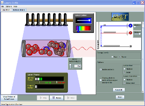
Figure 9:A two- and three-level laser with pump, mirrors, and output coupler. (This is one of PhET’s original Java simulations, run in the browser by CheerpJ; it downloads a Java runtime before it starts, so give it a few seconds on first load.) Build a population inversion and watch stimulated emission grow into a cavity mode.
Interactive simulation: Lasers
For electromagnetic energy density per unit of frequency interval, the rate equations are
Hence, for :
where as before: is constant. If initially (i.e. at ) all atoms are in the lowest state: , then it follows from Eq. (27):
An example where is shown in Figure 10. We always have , hence for all times . Therefore, this closed two-level system cannot develop population inversion when it is pumped only on the same transition.
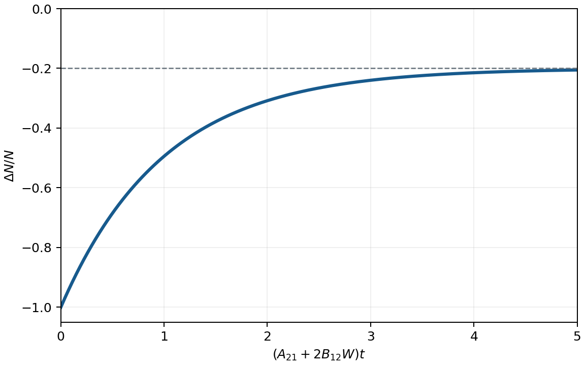
Figure 10: as a function of when all atoms are in the ground state at , i.e. .
A way to achieve population inversion between levels 1 and 2, and thus amplification at , is to use a third atomic level. In Figure 11 the ground state is state 1 with two upper levels 2 and 3 such that . The transition of interest is still that from level 2 to level 1. Initially almost all atoms are in the ground state 1. Then atoms are pumped with rate from level 1 directly to level 3. The transition is non-radiative and has a high rate so that level 3 is quickly emptied and therefore remains small. State 2 is called a metastable state, because the residence time of each atom in this state is relatively long. Therefore its population tends to increase, leading to population inversion between the metastable state 2 and the lower ground state 1 (which is continuously being depopulated by pumping to the highest level).
The direct relaxation rate should be small compared with so that pumping efficiently populates level 2. Because level 1 is the ground state, a three-level laser requires substantial pumping to deplete it before inversion occurs.
Pumping may be done optically as described, but the energy to transfer atoms from level 1 to level 3 can also be supplied by an electrical discharge in a gas or by an electric current. Spontaneous emission provides seed photons in the cavity modes. Once the gain exceeds losses, stimulated emission amplifies these photons and laser oscillation grows. Photons emitted into a resonant cavity mode can stimulate atoms in level 2 to decay to level 1, each adding a photon of energy to that mode. The stimulated emission enters the same mode with a fixed phase relation to the exciting light and hence the light amplitude continuously builds up coherently, while it is bouncing back and forth between the mirrors of the resonator. An output coupler transmits a fraction of the circulating light as useful laser output.
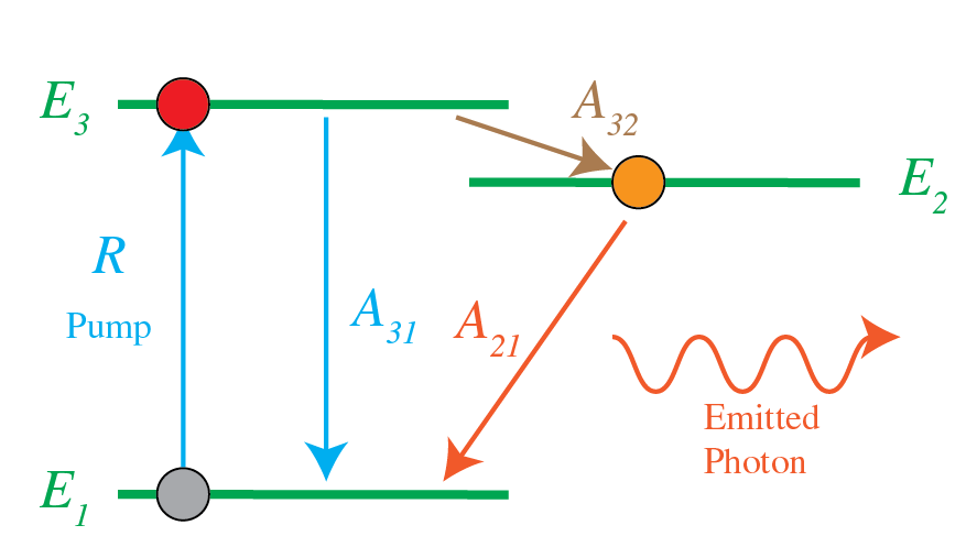
Figure 11:Three-level pumping scheme: level 1 to 3 pumping, rapid 3 to 2 relaxation, and 2 to 1 laser emission.
4Cavities
The amplifying medium can completely fill the space between the mirrors as at the top of Figure 12, or there can be space between the amplifier and the mirrors. For example, if the amplifier is a gas, it may be enclosed by a glass cylinder. Its end faces may be cut so that the intracavity beam meets them at Brewster incidence, as shown in the middle figure of Figure 12, to minimize reflections. This type of resonator is called a resonator with external mirrors.
Often one or both mirrors are concave toward the cavity, as in the bottom drawing of Figure 12. We state without proof that in that case the distance between the mirrors and the radii of curvature and of the mirrors has to satisfy
or else the laser light will ultimately leave the cavity laterally, i.e. it will escape sideways. This condition is called the stability condition. In this formula is positive for a mirror concave toward the cavity and negative for a convex mirror. Two concave mirrors can form a stable cavity when their radii and spacing satisfy the stated inequality; limiting cases require separate treatment.
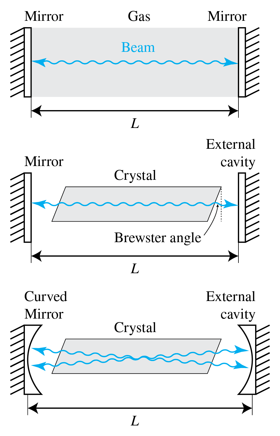
Figure 12:Three types of laser cavity. The shaded region is the amplifier. The middle case is called a laser with external mirrors.
5Problems with Laser Operation
In this section we consider some problems that occur with lasers and discuss what can be done to solve them.
Multiple Resonance Frequencies
In many applications such as laser communication and interferometry one needs a single wavelength. Consider a cavity of length as shown in Figure 13 and suppose that the amplifier has a gain curve covering many resonances of the resonator. One way to achieve single-frequency output is by taking care that there is only one frequency for which the gain is larger than the losses. One then says that the laser is above threshold for only one frequency. This can be done by choosing the length of the cavity to be so small that there is only one mode under the gain curve for which the gain is higher than the losses. However, a small length of the amplifier means less output power and a less collimated output beam. Another method would be to reduce the pumping so that for only one mode the gain compensates the losses. But this implies again that the laser output power is relatively small. A better solution is to add a Fabry-Perot cavity inside the laser cavity as shown in Figure 14. The added Fabry–Pérot etalon has optical thickness . Its approximate free spectral range at normal incidence is ; for a glass plate of physical thickness and refractive index , . Choosing a small optical thickness can leave only one etalon transmission peak under the amplifier gain curve. Furthermore, by choosing the proper angle for the Fabry-Perot cavity with respect to the axis of the laser cavity, the Fabry-Perot resonance can be coupled to the desired resonance frequency.
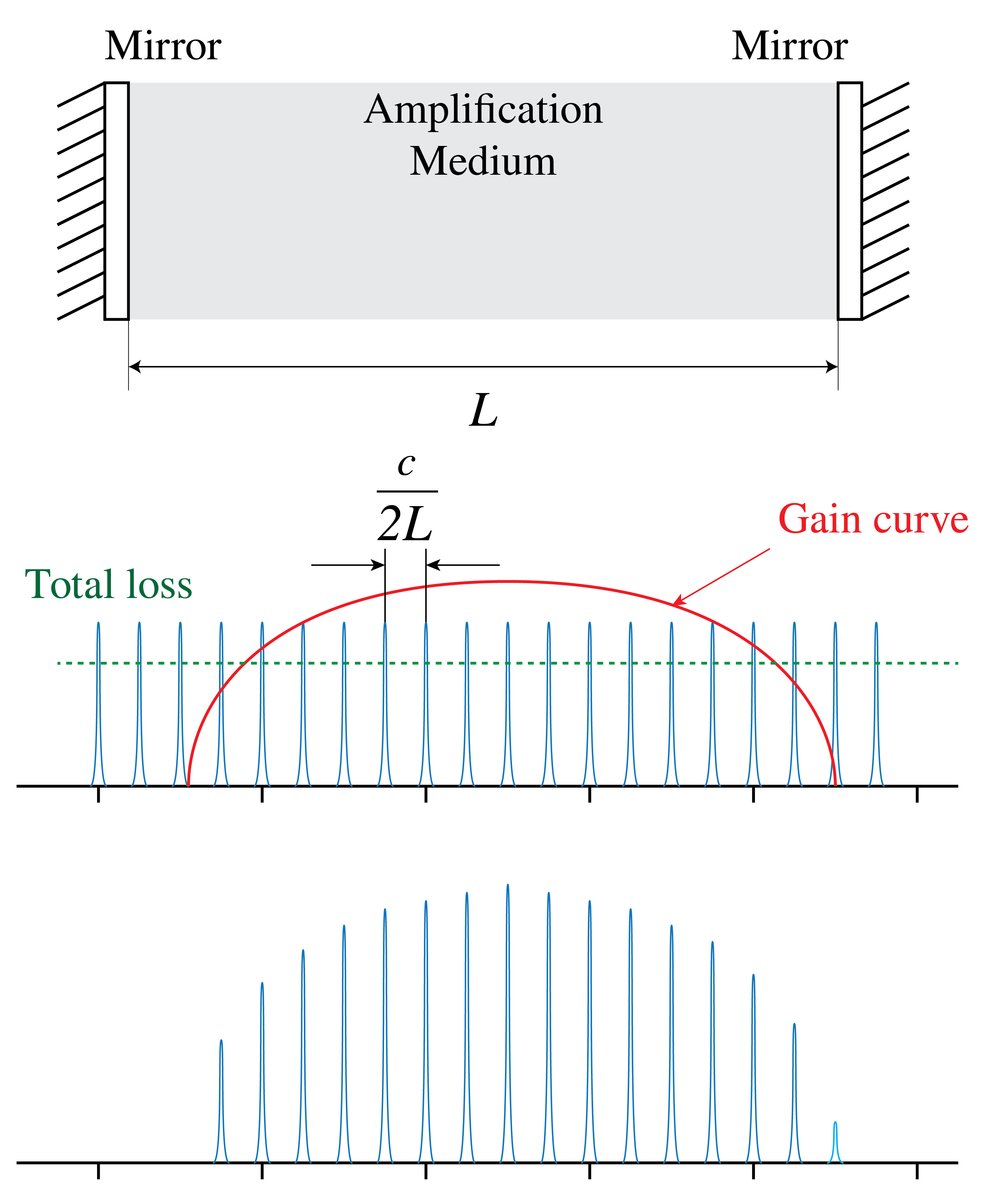
Figure 13:Laser with cavity of length and broad amplifier gain curve. Many resonance frequencies are above threshold to compensate the losses.
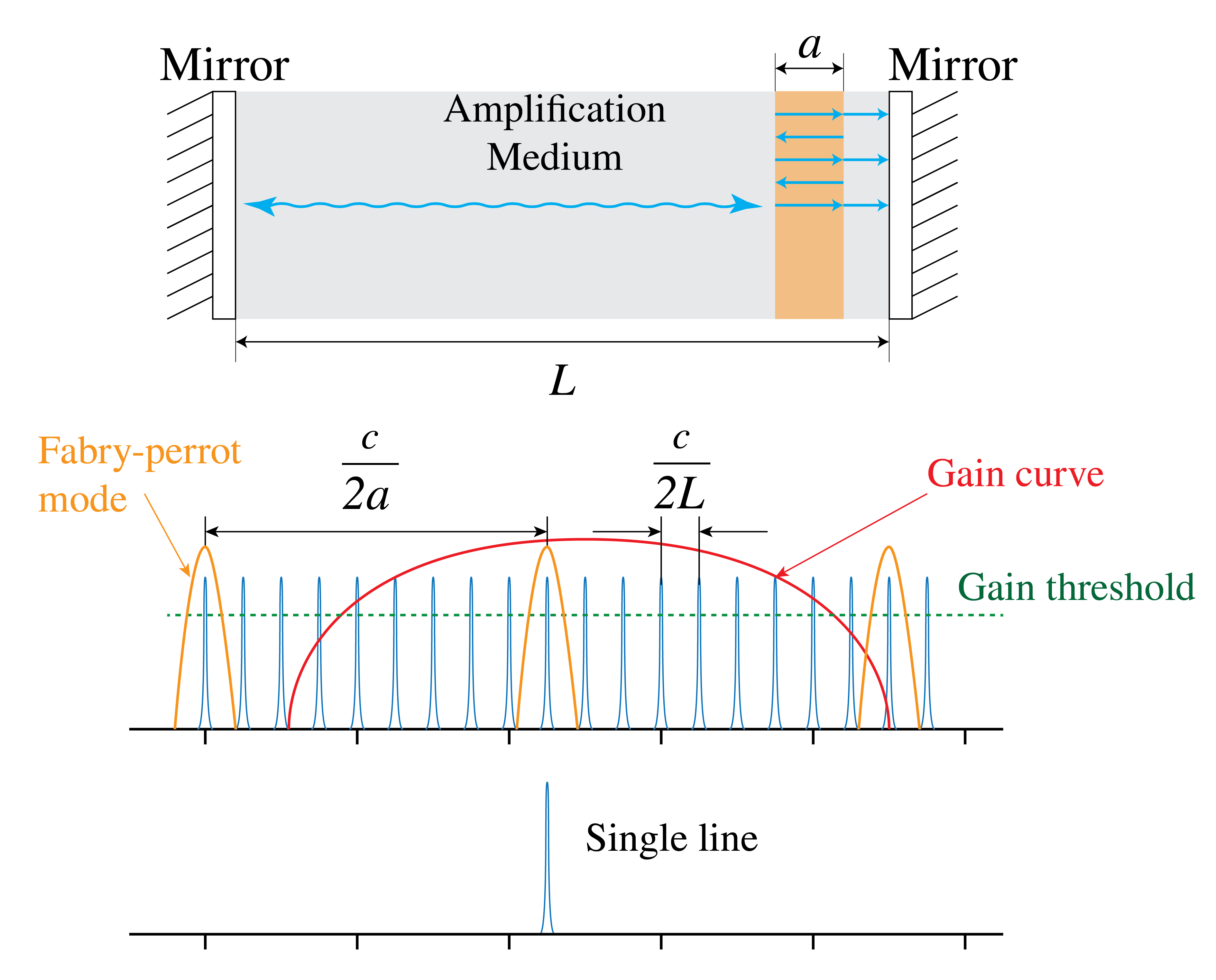
Figure 14:Laser with cavity of length , a broad amplifier gain curve and an added Fabry-Perot cavity. The Fabry-Perot resonances act as an extra filter to select only one mode of the laser.
Multiple Transverse Modes
A common laser mode has a Gaussian transverse intensity distribution. The Gaussian transverse pattern is the fundamental TEM transverse mode. Its standing-wave resonance has a longitudinal mode index ; in the plane-wave approximation for an air-filled cavity, . However, inside the laser cavity other modes with different transverse patterns can also resonate. An example is shown in Figure 15 where TEM has two intensity maxima.
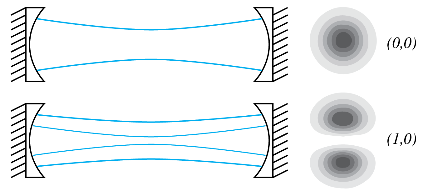
Figure 15:Laser cavity with (0,0) and (1,0) modes.
There exist many more transverse modes, as shown in Figure 16. Different transverse families generally have slightly different resonance frequencies. So even when only one longitudinal index is above threshold for TEM, there can be many transverse modes with frequencies very close to the frequency of the Gaussian mode, which are also above threshold. This is illustrated in Figure 17 where the frequencies of modes (0,0), (1,0) and (1,1) all are above threshold.
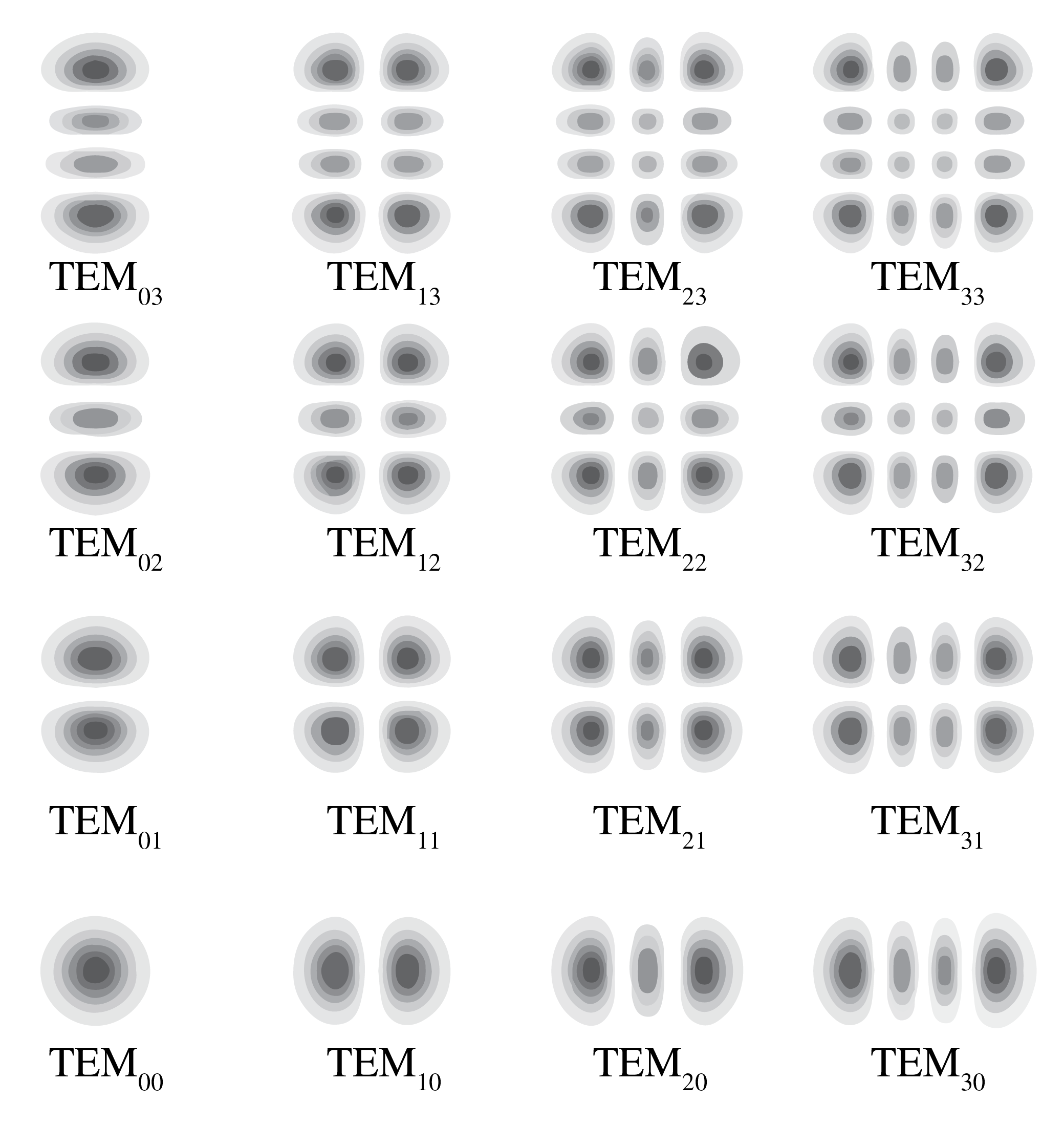
Figure 16:Intensity pattern of several transverse modes.
For a smooth, focusable beam, the fundamental Gaussian transverse mode is often preferred over higher-order modes. Because TEM is concentrated closest to the optical axis, a suitably chosen intracavity aperture can give higher-order transverse modes greater loss and favor fundamental-mode operation.
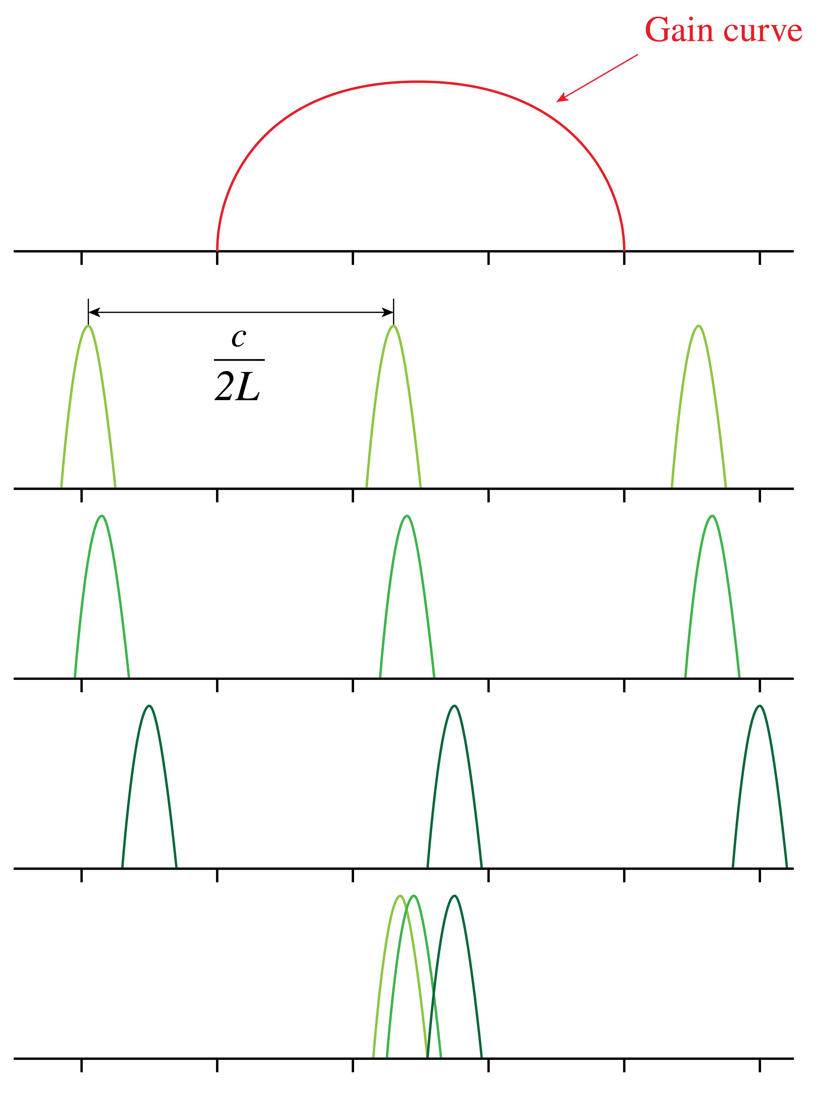
Figure 17:Resonance frequencies of transverse modes that have sufficient gain to compensate the losses.
6Types of Lasers
There are many types of lasers: gas, solid, liquid, semiconductor, chemical, excimer, e-beam, free electron, fiber and even waveguide lasers. We classify them according to the pumping mechanism.
6.1Optical Pumping
The energy to transfer the atom from the ground state to the excited state is provided by light. The source could be another laser or an incoherent light source, such as a discharge lamp. If is the atom in the ground state and is the excited atom, we have
where is the frequency for the transition as seen in Figure 18. The ruby laser, using chromium-doped , was the first demonstrated laser in 1960. It emits pulses of light of wavelength 694.3 nm and is optically pumped with a gas discharge lamp. Other examples include Nd:YAG, doped-glass, fiber, and dye lasers; some semiconductor lasers can also be optically pumped.
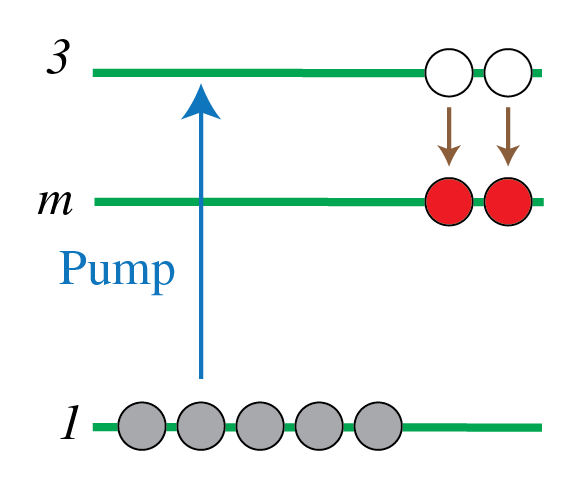
Figure 18:Population transfer in an optically pumped laser: the pump raises atoms from level 1 to level 3, and a rapid transition feeds metastable level , where atoms can accumulate.
In a dye laser the gain medium is a liquid dye, such as Rhodamine 6G. An external light source pumps it; the broad gain spectrum allows tuning over a range of wavelengths. We can select a certain wavelength by inserting a dispersive element like the Fabry-Perot cavity inside the laser cavity and rotating it at the right angle to select the desired wavelength, as explained above.
6.2Electron-Collision Pump
Energetic electrons are used to collide with the atoms of the amplifier, thereby transferring some of their energy:
where means an electron with energy and where is equal to so that the atom is transferred from the ground state 1 to state 3 to obtain population inversion. Examples include some argon, krypton, nitrogen, and copper vapor lasers. In a He–Ne laser the discharge primarily excites helium, which transfers energy to neon through collisions. Electrons can be created by a discharge or by an electron beam.
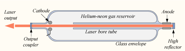
Figure 19:He–Ne laser schematic with a discharge bore, gas reservoir, cathode and anode; the output coupler and high reflector form the cavity (from Wikimedia Commons by DrBob / CC BY-SA 3.0).
6.3Atomic Collision
Let be atom in an excited, so-called metastable state. This means that , although unstable, has a very long relaxation time, i.e. longer than 1 ms or so. If collides with atom , it transfers energy to .
is the excited state used for the stimulated emission. If is the relaxation time of metastable state , then is very large and hence the spontaneous emission rate is very small. This implies that the number of metastable atoms as a function of time is given by a slowly decaying exponential function .
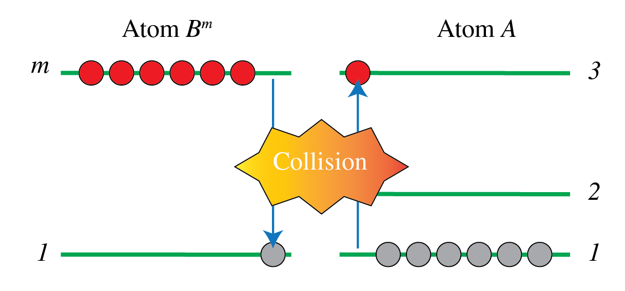
Figure 20:Pumping atoms to an excited state by collision with metastable atoms .
To get metastable atoms, one can for example pump atom B from its ground state 1 to an excited state 3 above state m such that the spontaneous emission rate is large. The pumping can be done electrically or by any other means. If it is done electrically, then we have
Examples of these types of laser are He–Ne, which commonly emits red light near 632.8 nm, N-CO and He-Cd. Energy-transfer collisions are important in these examples, but the pumping and lasing transitions differ among the gas mixtures. The CO laser emits near 10.6 m and can achieve huge power.
6.4Chemical Pump
In some chemical reactions, a molecule is created in an excited state with population inversion. An example is:
So in this case the lasing will take place for a transition between states of molecule . HF is an example of a chemically pumped laser. Excimer lasers such as ArF and XeCl use different discharge-driven mechanisms.
6.5Semiconductor Laser
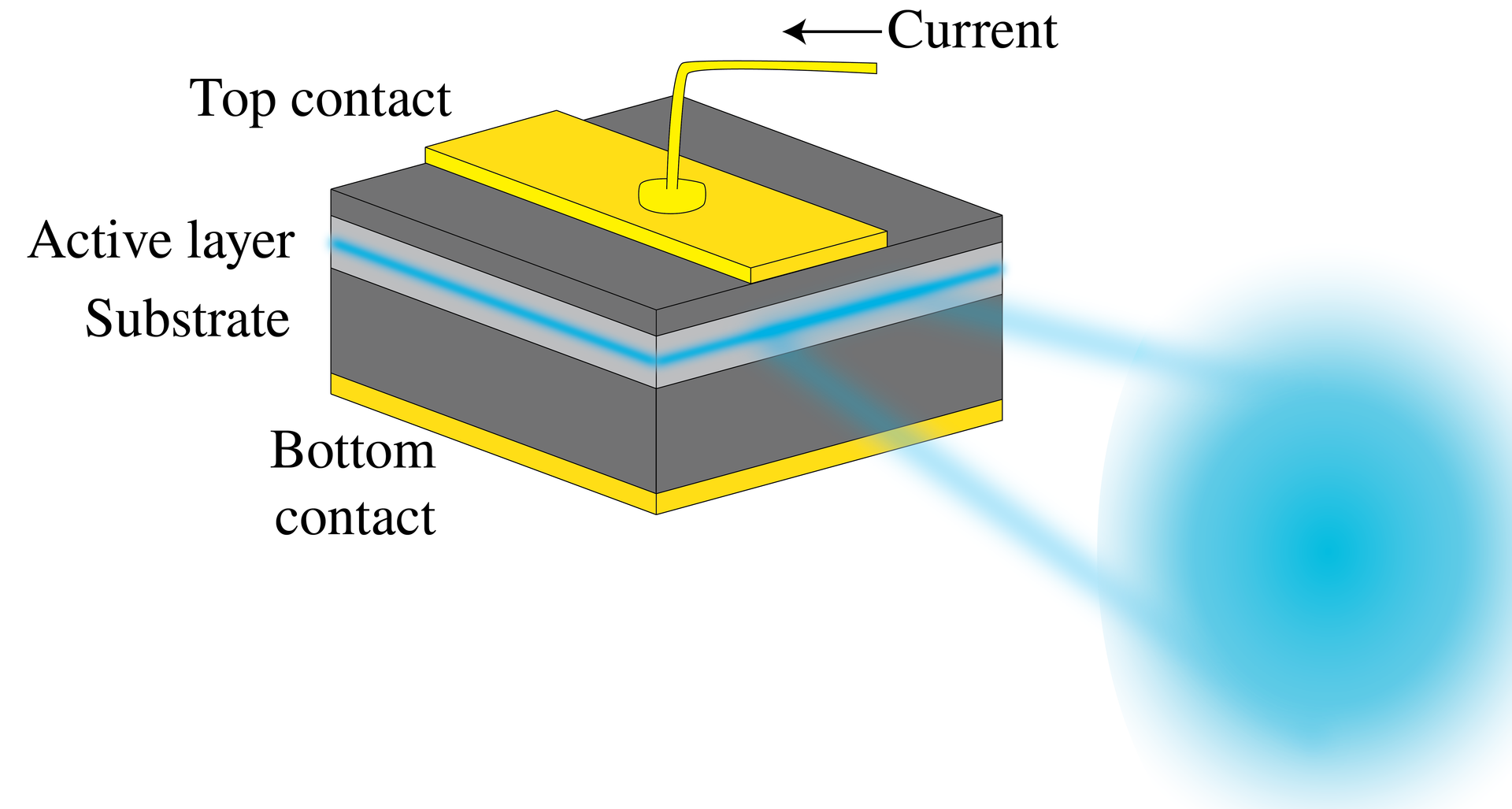
Figure 21:Surface-emitting semiconductor laser: current enters through the top contact and recombination in the active layer produces a beam normal to the chip surface.
In the surface-emitting semiconductor laser shown in Figure 21, electrical current injects electrons and holes into an active region, where recombination provides optical gain. The beam leaves approximately perpendicular to the chip surface. A vertical-cavity surface-emitting laser (VCSEL) uses mirrors above and below this region, typically distributed Bragg reflectors. This geometry differs from an edge-emitting diode laser, whose cavity runs along the chip and whose output leaves an edge.
7Chapter Summary
Laser stands for Light Amplification by Stimulated Emission of Radiation.
Key laser properties: High intensity, monochromaticity, directionality (low divergence), and high temporal and spatial coherence.
Einstein coefficients describe absorption (), stimulated emission (), and spontaneous emission ().
Population inversion () is essential for amplification; it cannot occur in thermal equilibrium.
Optical resonator (cavity): Two mirrors select specific longitudinal modes; mode spacing is .
Gain medium amplifies light through stimulated emission; the gain curve depends on the medium’s energy levels.
Threshold condition: Gain must exceed losses (mirror transmission, scattering, absorption) for lasing.
Three-level systems: Pumping must deplete the ground state enough for the upper laser level to become more populated.
Transverse modes (TEM): Higher-order modes have more complex spatial profiles; often suppressed for beam quality.
Pumping mechanisms: Optical (flashlamp, diode laser), electrical (gas discharge, current injection), or chemical.
Laser types: Solid-state (Nd:YAG, Ruby), gas (He-Ne, CO), semiconductor (diode lasers), and dye lasers.