This chapter provides a comprehensive introduction to the nature of light, covering its historical development, wave-particle duality, the electromagnetic spectrum, and radiometry. It establishes the foundational concepts necessary for understanding optical phenomena and technologies discussed in later chapters.
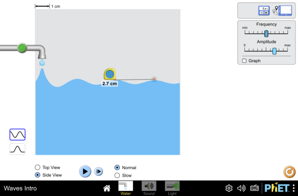
Figure 1:The simulation shows a single oscillating source drawn as a water wave, a sound wave, or a light wave. Use it to connect the shared language of wavelength, frequency, and propagation speed before the particle picture introduced later in the chapter.
Interactive simulation: Waves Intro
0.1Introduction
Light permeates every aspect of human existence. Vision, our most treasured sensory faculty, allows light to inspire profound emotional responses—whether we’re witnessing a breathtaking sunset or catching sight of a rainbow emerging through storm clouds. Beyond evoking wonder, light serves countless practical purposes: entertaining audiences in theaters, signaling drivers at traffic lights, transmitting telephone communications through optical fibers, and providing energy for solar cooking. Light’s energy forms the foundation of life itself, from enabling photosynthesis in plants to providing warmth for cold-blooded creatures.
While we understand that visible light consists of electromagnetic waves detectable by human eyes, numerous fundamental questions about light and vision remain. What creates color, and how do our visual systems perceive it? What causes diamonds to exhibit their characteristic brilliance? How does light propagate through space? What mechanisms allow lenses and mirrors to create images? The field of optics addresses these questions and many others.
Light has been one of physics’ most fascinating challenges; even 60 years after early quantum discoveries, Einstein admitted we were still in a state of “learned ignorance” about light’s true nature. In fact, light connects multiple physics disciplines - optics, electricity, magnetism, and atomic physics - representing one of the great unifications in our understanding of the physical world.
0.2A Brief History
The scientific understanding of light has undergone a remarkable evolution spanning more than three centuries, shaped by competing theories, groundbreaking experiments, and revolutionary insights that fundamentally changed our view of physical reality. This journey from classical mechanics to quantum theory represents one of the most profound intellectual transformations in the history of science, revealing the subtle and counterintuitive nature of light itself.
In the 17th century, Isaac Newton proposed an influential particle theory: light consisted of tiny “corpuscles” traveling along paths that could explain sharp shadows and reflection. He modeled refraction through forces acting near an interface. Thin-film colors, including the rings produced by a curved lens on a flat plate, required additional assumptions. Newton studied these rings in detail, though he did not interpret them as evidence for a wave theory. His particle account remained influential for more than a century.
Contemporary with Newton but representing a fundamentally different philosophical approach, the Dutch physicist Christiaan Huygens advanced a sophisticated wave theory of light that would prove remarkably prescient. Huygens proposed that light propagated as waves through an all-pervading, invisible medium called the “luminiferous ether,” much as sound waves travel through air or water waves move across the ocean’s surface. According to Huygens’ principle, every point on an advancing wavefront could be considered as a source of secondary wavelets, and the envelope of these wavelets determined the new position of the wavefront as it propagated through space. This elegant geometric construction successfully explained not only the familiar phenomena of reflection and refraction but also more complex behaviors that challenged Newton’s particle theory. Huygens’ construction also addressed double refraction in calcite, where an incident beam splits into two rays; their distinct polarizations were understood later. The superposition of crossing light beams is natural in a linear wave model.
The early 19th century witnessed a decisive shift in scientific opinion with Thomas Young’s ingenious double-slit experiment, an investigation that many consider one of the most beautiful and profound experiments in the history of physics. Young directed light through two closely spaced, parallel slits and observed the resulting pattern on a screen placed behind the slits. Instead of seeing two bright bands corresponding to light passing through each slit—as particle theory would predict—Young observed a series of alternating bright and dark fringes, a characteristic interference pattern that could only be explained if light behaved as waves. The bright fringes occurred where waves from the two slits arrived in phase, reinforcing each other through constructive interference, while the dark fringes appeared where the waves arrived out of phase, canceling each other through destructive interference. This elegant demonstration provided compelling, virtually irrefutable evidence for the wave nature of light and shifted the scientific consensus decisively away from Newton’s particle theory toward Huygens’ wave model. Young’s experiment also allowed for the first accurate measurements of light’s wavelength, revealing that different colors corresponded to different wavelengths, with red light having longer wavelengths than blue light, providing a physical basis for understanding the spectrum of colors that had fascinated natural philosophers since Newton’s work with prisms.
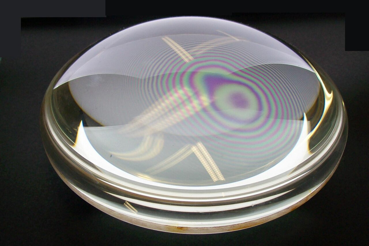
Figure 2:Newton’s rings arise from interference between reflections at the two surfaces of the thin air gap. Its thickness increases away from contact. One reflected ray reverses phase, so a zero-thickness contact is dark in reflected monochromatic light; successive bright and dark rings follow as the round-trip path changes. White light gives the colored rings in the photograph. Their radii depend on wavelength and surface curvature.
The triumph of wave theory in the early 1800s sparked a period of remarkable theoretical and experimental progress that would define 19th-century optics. Augustin Fresnel made fundamental contributions to understanding polarized light, demonstrating that light waves were transverse rather than longitudinal—meaning that the oscillations occurred perpendicular to the direction of propagation, like waves on a string, rather than parallel to it, like sound waves in air. Fresnel’s mathematical analysis of polarization phenomena led to his famous equations, which accurately predicted the fraction of light reflected and transmitted when electromagnetic waves encounter interfaces between materials with different optical properties. These equations became cornerstone tools for optical design and engineering, enabling the development of sophisticated optical instruments and technologies. Meanwhile, experimental investigations revealed increasingly subtle wave phenomena, including circular and elliptical polarization, optical activity in certain crystals and solutions, and the precise mathematical relationships governing diffraction patterns created by various apertures and obstacles. The wave theory seemed to provide a complete and satisfying account of all optical phenomena, requiring only the assumption of an ether medium to support the propagation of light waves through apparently empty space.
The intellectual culmination of 19th-century wave theory came with James Clerk Maxwell’s revolutionary electromagnetic theory, developed in the 1860s, which unified electricity, magnetism, and light into a single, elegant theoretical framework. Maxwell’s equations predicted that oscillating electric and magnetic fields could propagate through space as self-sustaining electromagnetic waves, with the electric and magnetic components oscillating perpendicular to each other and to the direction of propagation. Most remarkably, Maxwell found a wave speed close to the measured speed of light using independently measured electrical and magnetic constants. This mathematical prediction, confirmed by subsequent measurements, established that light was simply electromagnetic radiation within a specific frequency range, visible to human eyes by evolutionary accident rather than fundamental physical necessity. Maxwell’s theory implied the existence of electromagnetic radiation spanning a vast spectrum of frequencies, from radio waves with wavelengths of kilometers to gamma rays with wavelengths smaller than atomic nuclei, with visible light occupying only a tiny sliver of this electromagnetic spectrum. The experimental confirmation of radio waves by Heinrich Hertz in the 1880s provided dramatic validation of Maxwell’s theoretical predictions and seemed to establish electromagnetic wave theory as one of the great triumphs of 19th-century physics.
However, the dawn of the 20th century brought a series of experimental discoveries that would shatter the comfortable certainty of classical wave theory and usher in the quantum revolution that continues to shape modern physics. The crisis began with Max Planck’s investigation of blackbody radiation—the electromagnetic energy emitted by hot objects—which revealed that classical physics made predictions that disagreed dramatically with experimental observations. To resolve this “ultraviolet catastrophe,” Planck made the desperate assumption that energy could only be emitted or absorbed in discrete packets, or “quanta,” with energies given by , where was a new fundamental constant of nature (now called Planck’s constant) and was the frequency of the radiation. Although Planck initially viewed this quantization as a mathematical artifice rather than a fundamental feature of nature, his quantum hypothesis marked the beginning of a new era in physics that would revolutionize our understanding of light and matter.
Einstein’s explanation of the photoelectric effect provided the next crucial step in establishing the particle nature of light, earning him the Nobel Prize and helping to establish the reality of photons as discrete packets of electromagnetic energy. Einstein explained why, above a material-dependent threshold frequency, the maximum photoelectron kinetic energy depends on incident frequency, while intensity chiefly changes the emission rate. This follows from photons with energy . Each photon could transfer its entire energy to a single electron, providing enough energy to overcome the metal’s work function and eject the electron from the surface. Arthur Compton’s scattering experiments in the 1920s provided additional confirmation of photon reality by demonstrating that X-rays scattered from electrons behaved exactly like particles with momentum , experiencing billiard-ball-like collisions that conserved both energy and momentum according to relativistic mechanics.
The quantum revolution reached its philosophical climax with Louis de Broglie’s audacious proposal that the wave-particle duality observed in light was a universal feature of nature, extending to matter itself through the relationship , where matter particles with momentum should exhibit wave properties with wavelength . This hypothesis, initially met with skepticism, was dramatically confirmed by electron diffraction experiments that showed electrons creating interference patterns identical to those produced by light waves, revealing that the classical distinction between waves and particles was an artifact of limited experimental resolution rather than a fundamental feature of reality. The subsequent development of quantum mechanics by Schrödinger, Heisenberg, Born, and others established that all quantum objects—photons, electrons, atoms, and even large molecules—exhibit both wave and particle characteristics depending on how they are observed and measured, with the apparent contradiction resolved through the probabilistic interpretation of quantum mechanical wavefunctions that describe the likelihood of finding particles at particular locations when measurements are performed.
1Particles and Photons
The quantum mechanical revolution of the early 20th century fundamentally changed our understanding of light and matter. What emerged was a profound realization that neither the classical wave model nor the classical particle model alone could adequately describe the behavior of photons and electrons. Instead, these entities exhibit wave-particle duality—displaying both wave and particle characteristics depending on the experimental context in which they are observed.
1.1Wave-Particle Duality
The concept of wave-particle duality represents one of the most counterintuitive yet essential principles in modern physics. When we observe light in certain experiments, such as interference and diffraction phenomena, it behaves unmistakably like a wave. The famous double-slit experiment demonstrates this beautifully, producing interference patterns that can only be explained by wave superposition. However, in other contexts, such as the photoelectric effect or Compton scattering, light behaves as discrete particles called photons, each carrying a specific quantum of energy.
Similarly, electrons and other material particles, traditionally viewed as solid, localized objects, also exhibit wave-like properties. Louis de Broglie’s revolutionary hypothesis proposed that all matter has an associated wavelength, leading to the development of electron microscopy and our modern understanding of atomic structure.
1.2Fundamental Quantum Mechanical Equations
Quantum mechanics provides a unified mathematical framework that describes both material particles and photons through a set of fundamental relationships. For any particle or photon, the following equations connect energy, momentum, mass, and other properties:
The relativistic energy-momentum relation gives us:
The de Broglie wavelength relates the wave and particle aspects:
The relativistic velocity can be expressed as:
These equations apply universally to both massive particles and massless photons, though they simplify considerably for the photon case.
1.3Photon Properties
For photons, which have zero rest mass (), the fundamental equations reduce to elegant, simpler forms. Setting in the relativistic energy-momentum relation yields:
This tells us that a photon’s momentum is directly proportional to its energy, with the speed of light as the proportionality constant.
The de Broglie wavelength for photons becomes:
This relationship directly connects the wave property (wavelength) with the particle property (energy) through Planck’s constant .
In vacuum, photons of every energy travel at :
This universal speed is one of the defining characteristics of electromagnetic radiation and forms the basis for Einstein’s special theory of relativity.
1.4Example 1-1: Electron and Photon Comparison
To illustrate these concepts, consider an electron with kinetic energy MeV. We can calculate its relativistic properties and compare them with a photon of the same total energy.
For the electron, the total energy is MeV. Using equation Eq. (1), the momentum is:
The de Broglie wavelength from equation Eq. (2) is:
The electron’s speed from equation Eq. (3) is:
For a photon with the same total energy (3.011 MeV), the momentum is , the wavelength is , and its vacuum speed is . Both wavelengths are on the picometer scale.
1.5Statistical Behavior
Beyond their individual properties, electrons and photons exhibit fundamentally different statistical behaviors that have profound implications for quantum systems. Electrons, being fermions with half-integer spin, obey Fermi-Dirac statistics. This means they are subject to the Pauli exclusion principle—no two electrons can occupy the same quantum state simultaneously. This principle governs the structure of atoms, the periodic table of elements, and the electrical properties of materials.
Photons, on the other hand, are bosons with integer spin and obey Bose-Einstein statistics. Unlike electrons, multiple photons can occupy the same quantum state without restriction. This property is crucial for understanding laser operation, where stimulated emission produces many photons in the same mode, creating the coherent, intense light characteristic of laser beams.
The statistical differences also manifest in other phenomena. The tendency of bosons to “cluster” in the same state leads to Bose-Einstein condensation at very low temperatures, while the exclusion principle for fermions results in degeneracy pressure that supports white dwarf stars against gravitational collapse.
1.6Implications and Applications
The wave-particle duality and quantum mechanical description of light and matter have revolutionized technology and our understanding of nature. Electron microscopy exploits the wave nature of electrons to achieve resolution far beyond optical microscopes. Quantum electronics relies on the particle nature of light in devices like photodiodes and photomultiplier tubes. Modern telecommunications uses both aspects—the wave nature for propagation and interference effects in fiber optics, and the particle nature for quantum cryptography and single-photon detection.
The unification provided by quantum mechanics demonstrates that what we perceive as fundamentally different phenomena—waves and particles—are actually complementary aspects of a deeper quantum reality. This duality extends beyond photons and electrons to all quantum entities, forming the foundation for our modern understanding of atomic physics, condensed matter physics, and quantum field theory.
2The Electromagnetic Spectrum
Electromagnetic radiation encompasses an enormous range of wavelengths and frequencies, from radio waves spanning kilometers to gamma rays with wavelengths smaller than atomic nuclei. Despite this vast diversity, all electromagnetic waves share fundamental properties and are unified by the same underlying physics.
2.1Basic Properties of Electromagnetic Waves
All electromagnetic waves, regardless of their wavelength or frequency, travel at the same speed in vacuum: m/s. This universal speed represents one of nature’s fundamental constants and forms the cornerstone of Einstein’s special relativity.
The relationship between wavelength and frequency is given by:
This simple equation reveals an inverse relationship: as wavelength increases, frequency decreases proportionally. The energy of electromagnetic radiation is quantized in units called photons, with each photon carrying energy:
where is Planck’s constant. This quantization means that electromagnetic waves can only gain or lose energy in discrete amounts proportional to their frequency.
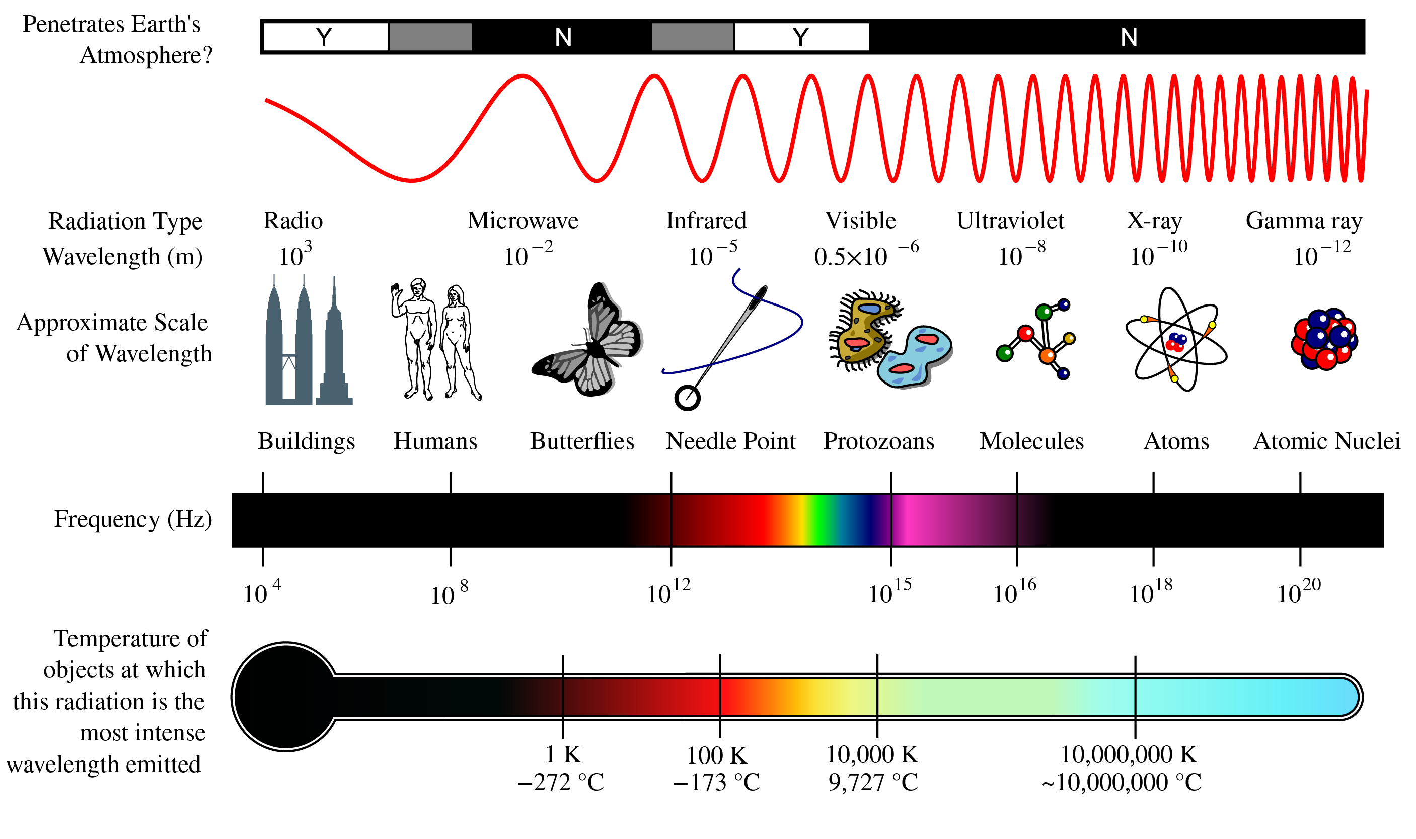
Figure 3:An overview of the electromagnetic spectrum, from radio through gamma rays. The illustrated wavelength and frequency axes cover roughly 15–16 orders of magnitude; the visible band is only a small interval. The region boundaries and atmospheric-transmission strip are schematic, not sharp limits.
2.2The Electromagnetic Spectrum Regions
The electromagnetic spectrum is traditionally divided into regions based on wavelength, frequency, and the physical mechanisms that produce and detect the radiation. Figure 1-1 illustrates these regions and their characteristic properties.
2.2.1Radio Waves
Radio waves represent the longest wavelengths in the electromagnetic spectrum, ranging from kilometers down to about one meter. These waves are produced by oscillating electric charges in antennas and circuits. Radio waves readily penetrate Earth’s atmosphere and can travel vast distances, making them ideal for communication. They are used in AM and FM radio broadcasting, television transmission, and various forms of wireless communication.
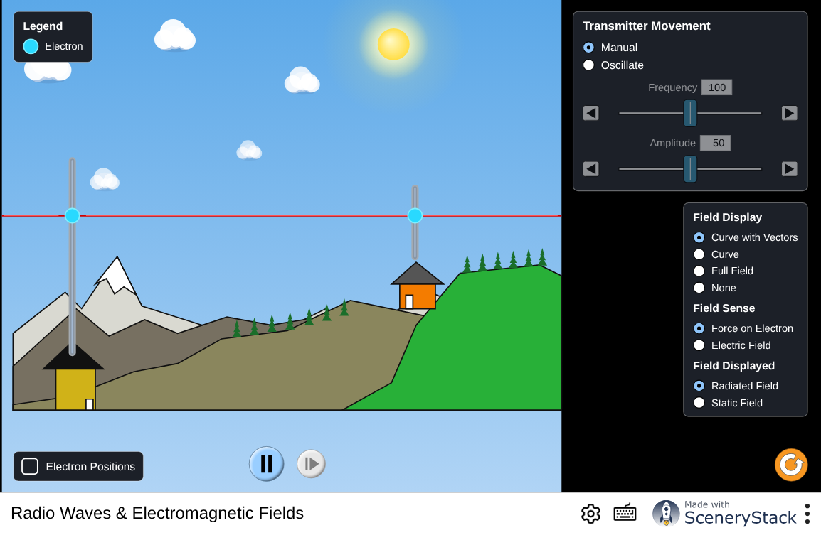
Figure 4:An accelerating charge and the electromagnetic disturbance it radiates. Move the charge and watch the fields propagate outward at — the classical picture behind radio transmission at the long-wavelength end of the spectrum.
Interactive simulation: Radio Waves
2.2.2Microwaves
With wavelengths from about one meter down to one millimeter, microwaves occupy the transition region between radio waves and infrared radiation. They are extensively used in radar systems, where their ability to reflect off objects enables distance and velocity measurements. Microwave ovens operate near 2.45 GHz; absorption by water and other polar or ionic components dissipates electromagnetic energy as heat. Satellite communications and cellular networks also use microwave bands.
2.2.3Infrared Radiation
Infrared (IR) radiation spans roughly 700 nanometers to one millimeter. Objects above absolute zero emit thermal radiation; warm objects emit substantial infrared radiation, while the peak wavelength depends on temperature according to Wien’s displacement law. Infrared radiation is subdivided into near-infrared (closest to visible light), mid-infrared, and far-infrared regions. Night-vision equipment detects infrared emission from warm objects, while infrared spectroscopy identifies molecular vibrations for chemical analysis.
2.2.4Visible Light
The visible portion of the electromagnetic spectrum represents only a tiny fraction of the total range, spanning roughly 380 to 750 nanometers, with perceptual limits varying between observers and conditions. Human eyes have evolved to detect this narrow band because it corresponds to the peak output of our Sun and the wavelengths that penetrate Earth’s atmosphere most effectively. Within this range, different wavelengths correspond to different colors: violet (380-450 nm), blue (450-495 nm), green (495-570 nm), yellow (570-590 nm), orange (590-620 nm), and red (620-770 nm).
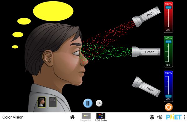
Figure 5:How the eye’s RGB cone responses combine, and how additive mixing of red, green, and blue light produces the colors we name in the visible band above.
Interactive simulation: Color Vision
2.2.5Ultraviolet Radiation
Ultraviolet (UV) radiation extends from the violet edge of visible light to shorter wavelengths. The commonly used biological bands are UV-A (315–400 nm), UV-B (280–315 nm), and UV-C (100–280 nm). The atmosphere absorbs solar UV-C and most UV-B before they reach the ground; artificial UV-C sources still pose exposure hazards. UV photons can drive chemical reactions and damage tissue. Ionization depends on both photon energy and the target, so it is not a property of every UV photon.
2.2.6X-rays
X-rays occupy wavelengths from about 10 nanometers down to 10⁻⁴ nanometers. They are typically produced when high-energy electrons bombard a metal target, causing the emission of characteristic X-rays as inner electron shells are disturbed. X-rays penetrate soft tissue but are absorbed by denser materials like bone, making them invaluable for medical imaging. X-ray crystallography uses the wave nature of X-rays to determine atomic structure in crystals through diffraction patterns.
2.2.7Gamma Rays
Gamma rays often have very short wavelengths and can originate in nuclear transitions and high-energy astrophysical processes. Their energies overlap those of X-rays; origin is often a more useful distinction than a fixed wavelength boundary. Shielding requirements depend on photon energy and source strength. In medicine, controlled gamma radiation is used for cancer treatment, while gamma-ray astronomy reveals the most energetic processes in the universe.
2.3Energy Quantization and Detection
A crucial concept for understanding electromagnetic radiation is that its energy becomes increasingly “grainy” at higher frequencies. Low-frequency radio waves have such small photon energies that individual photons are undetectable with ordinary instruments—the signal appears continuous. However, as frequency increases, photon energies become large enough that individual photons can be detected and counted.
2.4Example 1-2: Radar Detection and Photon Statistics
Consider a radar receiver detecting electromagnetic radiation at different wavelengths. For a 10-meter radio wave (30 MHz), each photon carries energy J. A 10-12 W received signal at this frequency corresponds to about photon energies per second. Ordinary radar measures the collective electromagnetic field rather than resolving single microwave photons.
In contrast, 0.1 nm X-ray photons have energy J, about 1011 times the radio photon energy. If the received X-ray power were also 10-12 W, it would deliver about 500 photons per second to a detector with perfect collection and detection efficiency.
Photon energy changes the number of photons at a fixed received power; it does not by itself determine telescope size. Radio dishes also need collecting area for faint sources and aperture for angular resolution, while X-ray telescopes require suitable focusing optics and photon-sensitive detectors.
The electromagnetic spectrum thus represents a continuum of radiation unified by common physical principles yet displaying remarkably diverse properties and applications across its vast range of wavelengths and frequencies.
3The Speed of Light
The speed of light in vacuum, , is a defining SI constant. Inertial observers measure the same vacuum value. In a material, phase velocity depends on frequency and the medium; pulse or signal propagation can involve a different group velocity.
3.1Historical Measurements of Light’s Speed
3.1.1Roemer’s Astronomical Method
The first strong evidence for a finite light-travel time came from Io’s eclipses. In 1676, Danish astronomer Ole Rømer (1644–1710) observed that eclipse times accumulated a delay when Earth was moving away from Jupiter and an advance when it was approaching. Io’s orbital period was not changing by the accumulated amount.
Roemer’s brilliant insight was recognizing that this fluctuation resulted from light’s finite travel time. When Earth moved away from Jupiter in its orbit, light from Io’s eclipses had to travel greater distances to reach terrestrial observers. Conversely, when Earth approached Jupiter, the light path shortened, causing eclipses to appear to occur earlier than predicted.
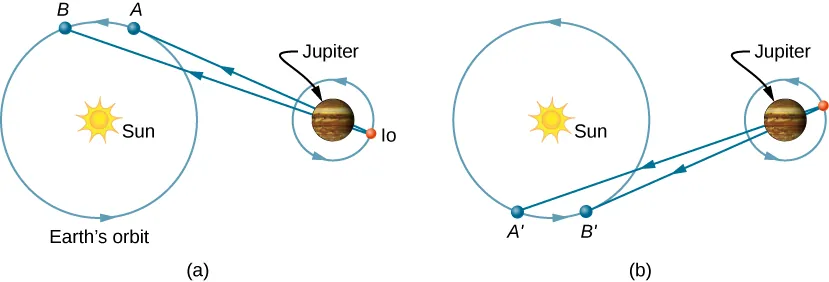
Figure 6:Roemer’s method for measuring the speed of light using observations of Io’s eclipses. The apparent timing of eclipses varies as Earth’s distance from Jupiter changes throughout the year.
Rømer’s timing argument established that light takes time to cross the changing Earth–Jupiter distance. A historical estimate using the then-known planetary distances was about , roughly one-third below the modern value.
3.1.2Terrestrial Measurements
The first successful Earth-based measurement came in 1849 from French physicist Armand Fizeau (1819–1896). His ingenious apparatus consisted of a rapidly rotating toothed wheel placed on one hilltop, with a mirror positioned 8 kilometers away on another hilltop. As the wheel rotated, it chopped a light beam into pulses. Fizeau adjusted the wheel’s rotation speed until no reflected light returned to the observer—this occurred when the wheel rotated just enough for a tooth to block the returning light pulse.
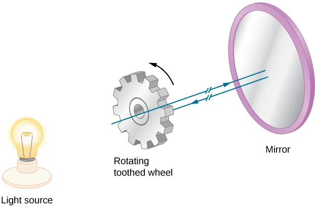
Figure 7:Fizeau’s rotating wheel method. Light passes through the gaps between the teeth to reach the mirror, but returning light is blocked when the wheel rotates at the correct speed.
From the wheel’s rotation rate, the number of teeth, and the distance to the mirror, Fizeau calculated light’s speed as —only 5% higher than the accepted value.
Jean Bernard Léon Foucault (1819–1868) refined this approach by replacing the toothed wheel with a rotating mirror, achieving even greater accuracy. By 1862, he measured the speed of light as , within 0.6% of today’s accepted value.
Albert Michelson (1852–1931) continued refining optical speed measurements. His 1926 result was reported as , with the uncertainty expressed in kilometers per second.
3.2The Modern Value
Since the 1983 definition of the metre, the speed of light in vacuum has this exact SI value:
The approximate value of provides sufficient accuracy for most calculations requiring three-digit precision.
3.3Speed of Light in Matter
When light travels through materials other than vacuum, it slows down due to interactions with atoms in the medium. This interaction varies significantly among different materials, depending on their atomic structure, crystal lattices, and other microscopic properties.
3.3.1Index of Refraction
For a monochromatic wave in an isotropic material, the phase refractive index, , relates vacuum speed to phase velocity:
This definition describes motion of a constant-phase wavefront. It is the appropriate for the refraction and wavelength examples below. The group speed of a pulse generally differs in a dispersive medium.
For the transparent visible-light examples below, and . This is not a universal inequality: an X-ray phase index can be below one. In vacuum, exactly.
3.3.2Representative Values
Table 1:Index of Refraction for Various Media
Medium | Temperature/Pressure | Index of Refraction () |
|---|---|---|
Gases | 0°C, 1 atm | |
Air | 1.000293 | |
Carbon dioxide | 1.00045 | |
Hydrogen | 1.000139 | |
Oxygen | 1.000271 | |
Liquids | 20°C | |
Benzene | 1.501 | |
Ethanol | 1.361 | |
Water (fresh) | 1.333 | |
Solids | 20°C | |
Diamond | 2.419 | |
Glass (crown) | 1.52 | |
Ice | 0°C | 1.309 |
Quartz (crystalline) | 1.544 | |
Zircon | 1.923 |
Gases at ordinary pressure have indices close to 1 because their optical response per unit volume is small. This is a collective wave response, not a sequence of vacuum flights interrupted by atoms. For rough estimates in air, is often adequate; precision work uses wavelength, temperature, pressure, and humidity.
3.3.3Example: Speed of Light in Gemstones
Let’s calculate the speed of light in zircon, a material often used in jewelry as a diamond substitute.
Given:
Index of refraction for zircon: (Table 1)
Speed of light in vacuum:
Solution:
Rearranging Eq. (13) to solve for :
This speed is slightly larger than half the speed of light in vacuum—still incredibly fast by everyday standards, yet significantly reduced from light’s maximum speed.
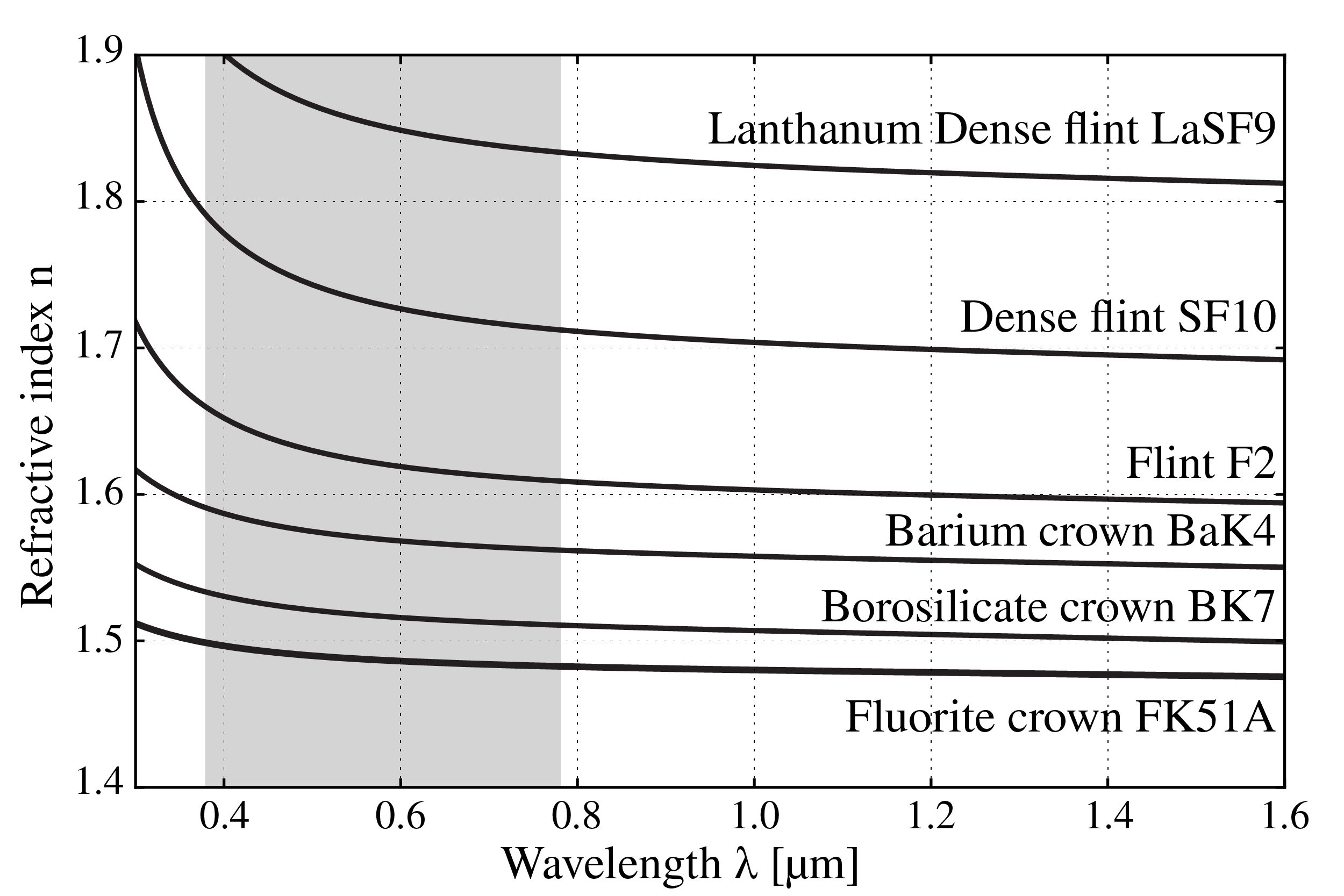
Figure 8:Refractive index as a function of wavelength for several types of glasses.
3.4The Ray Model of Light
Light can travel from a source to an observer through three primary pathways:
Direct propagation through empty space (such as sunlight reaching Earth)
Transmission through various media (such as light passing through air and glass)
Reflection from surfaces (such as light bouncing off a mirror)
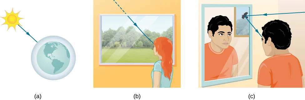
Figure 9:Three ways light can travel from source to observer: (a) direct transmission through vacuum, (b) transmission through media, and (c) reflection from surfaces.
3.4.1When Light Behaves as Rays
Experimental evidence shows that when light interacts with objects significantly larger than its wavelength, it travels in straight lines and behaves like rays. Since visible light has wavelengths less than one micrometer (10⁻⁶ m), it exhibits ray behavior when encountering most macroscopic objects we observe with unaided eyes.
In this ray model, light travels in straight lines until it encounters matter. Upon interaction, light may change direction—either by reflection (bouncing off surfaces) or refraction (bending when passing between different media)—but then continues traveling in straight lines.
3.4.2Geometric Optics
Since light rays follow straight-line paths and change direction according to geometric principles, we can describe light’s behavior using geometry and trigonometry. This branch of optics, called geometric optics, governs light’s interaction with matter through two fundamental laws:
Law of Reflection: Describes how light bounces off surfaces
Law of Refraction (Snell’s Law): Describes how light bends when passing between different media
These laws, combined with the ray model, provide powerful tools for analyzing optical systems ranging from simple mirrors to complex telescope designs.