1Introduction¶
In this chapter we will study how light propagates as a wave. In the study of the double-slit experiment we concluded from the interference pattern observed on a screen that light is a wave. To demonstrate more convincingly that light is indeed a wave, we require a detailed quantitative model of the propagation of light, which gives experimentally verifiable predictions.
But a precise description of the propagation of light is not only important for fundamental science; it also has many practical applications. For example, if a sample must be analyzed by illuminating it and measuring the scattered light, the fact that the detected light has been affected not only by the sample but also by propagation has to be taken into account. Another example is lithography. If a pattern has to be printed onto a substrate using a mask that is illuminated and there is a certain distance between the mask and the photoresist, the light which reaches the resist does not have the exact shape of the mask due to propagation effects. Thus, the mask needs to be designed to compensate for these effects.
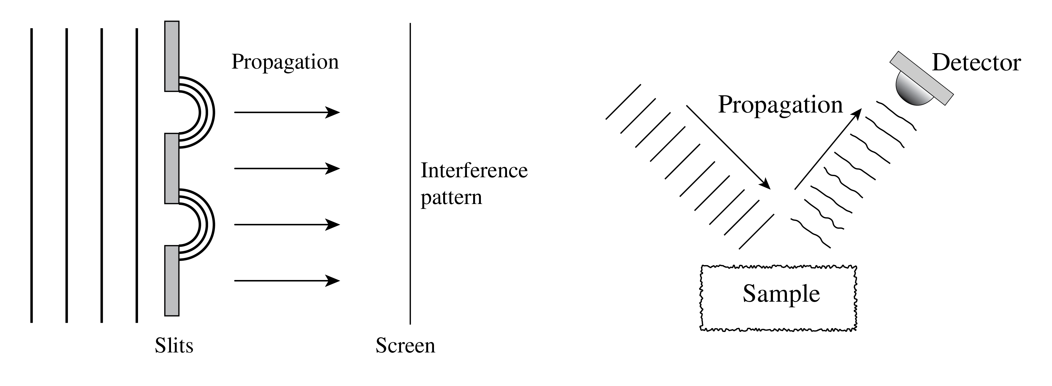
Figure 1:A quantitative model of the propagation of light is required to predict the properties of propagation and to apply it in sample analyses and lithography.
From electromagnetic theory, we know that in homogeneous matter (i.e. the permittivity is constant), every component of a time-harmonic electromagnetic field satisfies the scalar Helmholtz Eq. (1):
where is the wave number of the light in matter with permittivity and refractive index .
When the refractive index is not constant, Maxwell’s equations are no longer equivalent to the wave equation for the individual electromagnetic field components and there is then coupling between the components due to the curl operators in Maxwell’s equation. When the variation of the refractive index is slow on the scale of the wavelength, the scalar wave equation may still be a good approximation, but for structures that vary on a scale comparable to the wavelength, vector effects can make a scalar model inaccurate.
2Propagation of light through a homogeneous medium¶
We will describe two equivalent methods to compute the propagation of the field through homogeneous matter, namely the angular spectrum method and the Rayleigh-Sommerfeld diffraction formula. Our goal is to derive the field at some point with , given the field in the plane , as is illustrated in Figure 2. Although both methods ultimately describe the same propagation, they give physical insight into different aspects of propagation.
2.1Angular Spectrum Method¶
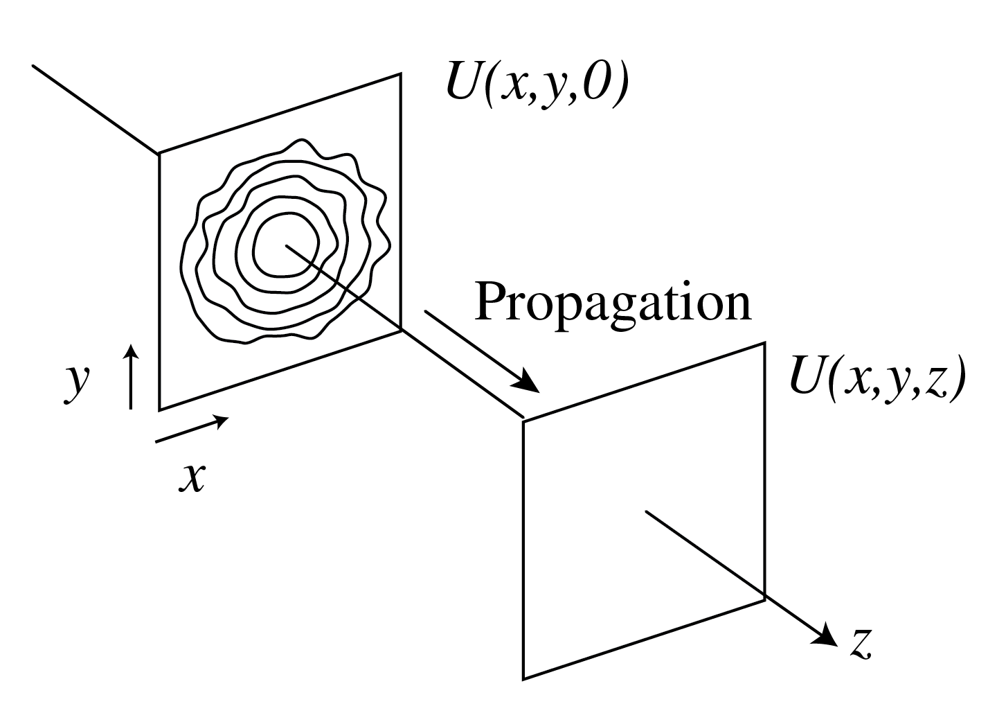
Figure 2:Given the field , we want to find at a point with . It is assumed that the field propagates in the positive -direction, which means that all sources are in the region .
The inverse Fourier transform implies:
The Fourier transform has important properties that are essential for this analysis. By defining , , Eq. (3) can be written as
The variables in the Fourier plane, and , are called spatial frequencies.
Eq. (4) says that we can write as an integral (a sum) of plane waves[1] with wave vector , each with its own weight (i.e. complex amplitude) . We know how each plane wave with complex amplitude and wave vector propagates over a distance
Therefore, the field in the plane (for some ) is given by
where
with the wavelength of the light as measured in the material (hence, , with the wavelength in vacuum). The sign in front of the square root in Eq. (7) could in principle be chosen negative: one would then also obtain a solution of the Helmholtz equation. The choice of the sign of is determined by the direction in which the light propagates, which in turn depends on the location of the sources and on the convention chosen for the time dependence. We have to choose here the + sign in front of the square root because the sources are in and the time dependence of time-harmonic fields is (as always in this book) given by with .
Eq. (6) can be written alternatively as
where now has to be considered as a function of :
Note that one can interpret this as a diagonalization of the propagation operator.
We can observe something interesting: if , then becomes imaginary, and decays exponentially for increasing :
These exponentially decaying waves are called evanescent in the positive -direction. We have met evanescent waves already in the context of total internal reflection. The physical consequences of evanescent waves in the angular spectrum decomposition are important for understanding diffraction limits.
The waves for which is real have constant amplitude: only their phase changes due to propagation. These waves therefore are called propagating waves.
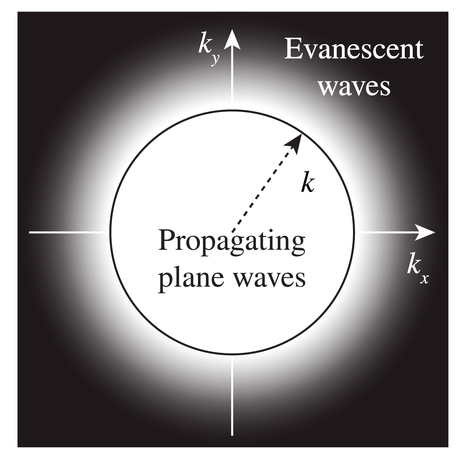
Figure 3:The spatial frequencies , of the plane waves in the angular spectrum of a time-harmonic field which propagates in the -direction. There are two types of waves: the propagating waves with spatial frequencies inside the circle and which have phase depending on the propagation distance but constant amplitude, and the evanescent waves for which and whose amplitude decreases exponentially during propagation.
Remark. In homogeneous source-free space, every electric-field component satisfies a scalar Helmholtz equation. The components must also obey Maxwell’s transversality condition. We may propagate each component , , and with the angular spectrum method if the starting fields satisfy that constraint. If the data in the plane of these field components are physically consistent, the electric field thus obtained will automatically satisfy the condition that the electric field is free of divergence, i.e.
everywhere in . This is equivalent to the statement that the electric vectors of the plane waves in the angular spectrum are perpendicular to their wave vectors. Alternatively, one can propagate only the - and -components and afterwards determine from the condition that Eq. (11) must be satisfied.
2.2Rayleigh-Sommerfeld Diffraction Integral¶
Another method to propagate a wave field is by using the Rayleigh-Sommerfeld integral. A very good approximation of this integral states that each point in the plane emits spherical waves with amplitude proportional to the field in the plane . To find the field at a point , we have to add the contributions from all these point sources together. This corresponds to the Huygens-Fresnel principle postulated earlier in the Spatial Coherence section of the Interference chapter. Because a more rigorous derivation starting from the Helmholtz equation[2] would be rather lengthy, we will just give the final result:
where we wrote again and where
Remarks.
The formula Eq. (12) is not completely rigorous because a term that is a factor smaller (and which in practice therefore is very much smaller) has been omitted.
In Eq. (12) there is an additional factor that has been omitted in the standard time-harmonic spherical wave formulation. This factor means that the amplitudes of the spherical waves in the Rayleigh-Sommerfeld diffraction integral depend on direction (although their wave fronts are spherical), the amplitudes being largest in the forward direction.
The angular spectrum method amounts to a multiplication by in Fourier space, while the Rayleigh-Sommerfeld integral is a convolution with respect to . It is a property of the Fourier transform that a multiplication in Fourier space corresponds to a convolution in real space and vice versa. Indeed a mathematical result called Weyl’s identity implies that the rigorous Rayleigh-Sommerfeld formulation and the plane wave expansion (i.e. the angular spectrum method) give identical results.
3Intuition for the Spatial Fourier Transform in Optics¶
Since spatial Fourier transformations play an important role in our discussion of the propagation of light, it is important to understand them not just mathematically, but also intuitively.
What happens when an object is illuminated and the reflected or transmitted light is detected at some distance from the object? Let us look at transmission for example. When the object is much larger than the wavelength, a transmission function is often defined and the field transmitted by the object is then assumed to be simply the product of the incident field and the function . For example, for a hole in a metallic screen with diameter large compared to the wavelength, the transmission function would be 1 inside the hole and 0 outside. However, if the object has features of the order of the wavelength, this simple model of multiplying by a transmission function breaks down and the transmitted field must instead be determined by solving Maxwell’s equations. This is not easy, but some software packages can do it.
Now suppose that the transmitted electric field has been obtained in a plane very close to the object (a distance within a fraction of a wavelength). This field is called the transmitted near field and it may have been obtained by simply multiplying the incident field with a transmission function or by solving Maxwell’s equations. This transmitted near field is a kind of footprint of the object. But it should be clear that, although it is quite common in optics to speak in terms of “imaging an object”, strictly speaking we do not image an object as such, but we image the transmitted or reflected near fields which are a kind of copy of the object. After the transmitted near field has been obtained, we apply the angular spectrum method to propagate the individual plane waves through homogeneous matter (e.g. air) from the object to the detector plane or to an optical element like a lens.
Let be a component of the transmitted near field. The first step is to Fourier transform it, by which the field component is decomposed into plane waves. To each plane wave, characterized by the wave numbers and , the Fourier transform assigns a complex amplitude , the magnitude of which indicates how important a role this particular wave plays in the formation of the near field. So what can be said about the object field , by looking at the magnitude of its spatial Fourier transform ?
Suppose has sharp features, i.e. there are regions where varies rapidly as a function of and . To describe these features as a combination of plane waves, these waves must also vary rapidly as a function of and , which means that the length of their wave vectors must be large. Thus, the sharper the features that has, the larger we can expect to be for large , i.e. high spatial frequencies can be expected to have large amplitude. Similarly, the slowly varying, broad features of are described by slowly fluctuating waves, i.e. by for small , i.e. for low spatial frequencies. This is illustrated in Figure 4.
To investigate these concepts further we choose a certain field, take its Fourier transform, remove the higher spatial frequencies and then invert the Fourier transform. We then expect that the resulting field has lost its sharp features and only retains its broad features, i.e. the image is blurred. Conversely, if we remove the lower spatial frequencies but retain the higher, then the result will only show its sharp features, i.e. its contours. These effects are shown in Figure 6. Recall that when , the plane wave decays exponentially as the field propagates. During propagation through homogeneous space, evanescent components are exponentially attenuated. At an ordinary far-field detector they are overwhelmed by noise, so conventional far-field imaging has limited resolution. Near-field methods can measure some of this detail before it decays.
It is this fact that motivates near-field microscopy, which tries to detect these evanescent waves by scanning close to the sample, thus obtaining subwavelength resolution.
So we have seen how we can guess properties of some object field given the amplitude of its spatial Fourier transform . But what about the phase of ? Although one cannot really guess properties of by looking at the phase of the same way as we can by looking at its amplitude, it is in fact the phase that plays a larger role in defining . This is illustrated in Figure 8: if the amplitude information of is removed, features of the original may still be retrieved. Knowing only Fourier magnitude generally does not uniquely determine the original field. Additional measurements or constraints can sometimes recover the phase. Thus, the phase of a field is very important, arguably often more important than its amplitude. However, we cannot measure the phase of a field directly, only its intensity from which we can calculate the amplitude . It is this fact that makes phase retrieval an entire field of study on its own: how can we find the phase of a field, given that we can only perform intensity measurements? This question is related to a new field of optics called “lensless imaging”, where amplitudes and phases are retrieved from intensity measurements and the image is reconstructed computationally. Interesting as this topic may be, we will not treat it in these notes and refer instead to master’s courses in optics [3].
Remark. The importance of the phase for the field can also be seen by looking at the plane wave expansion Eq. (6). We have seen that the field in a plane can be obtained by propagating the plane waves by multiplying their amplitudes by the phase factors , which depend on the propagation distance . If one leaves the evanescent waves out of consideration (since after some distance they hardly contribute to the field anyway), it follows that only the phases of the plane waves change upon propagation, while their amplitudes (the moduli of their complex amplitudes) do not change. Yet, depending on the propagation distance , widely differing light patterns are obtained (see e.g. Figure 12).
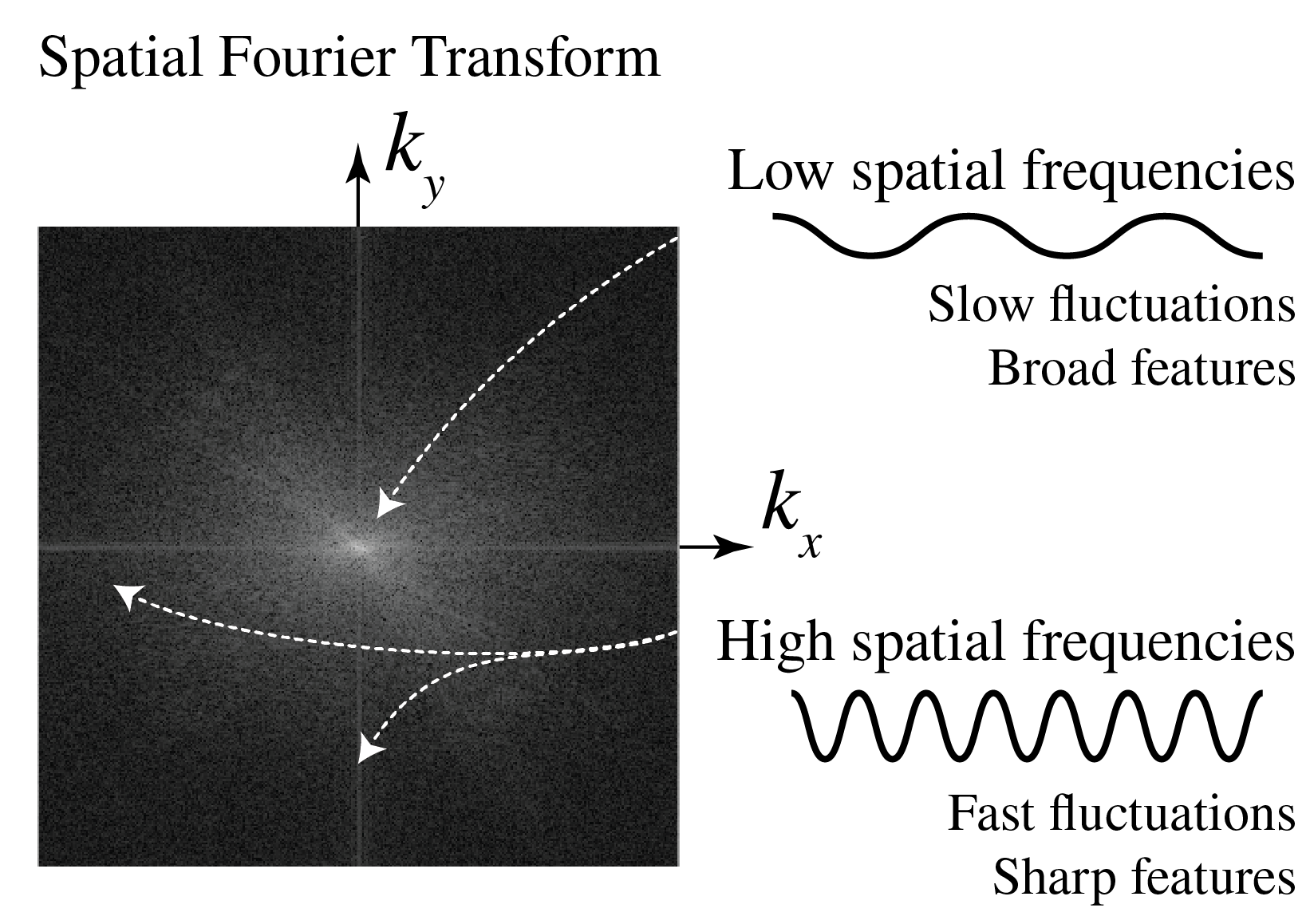
Figure 4:A qualitative interpretation of spatial Fourier transforms. The low spatial frequencies (i.e. small ) represent slow fluctuations, and therefore contribute to the broad features of the real-space object. The high spatial frequencies (i.e. large ) fluctuate rapidly, and can therefore form sharp features in the real-space object.
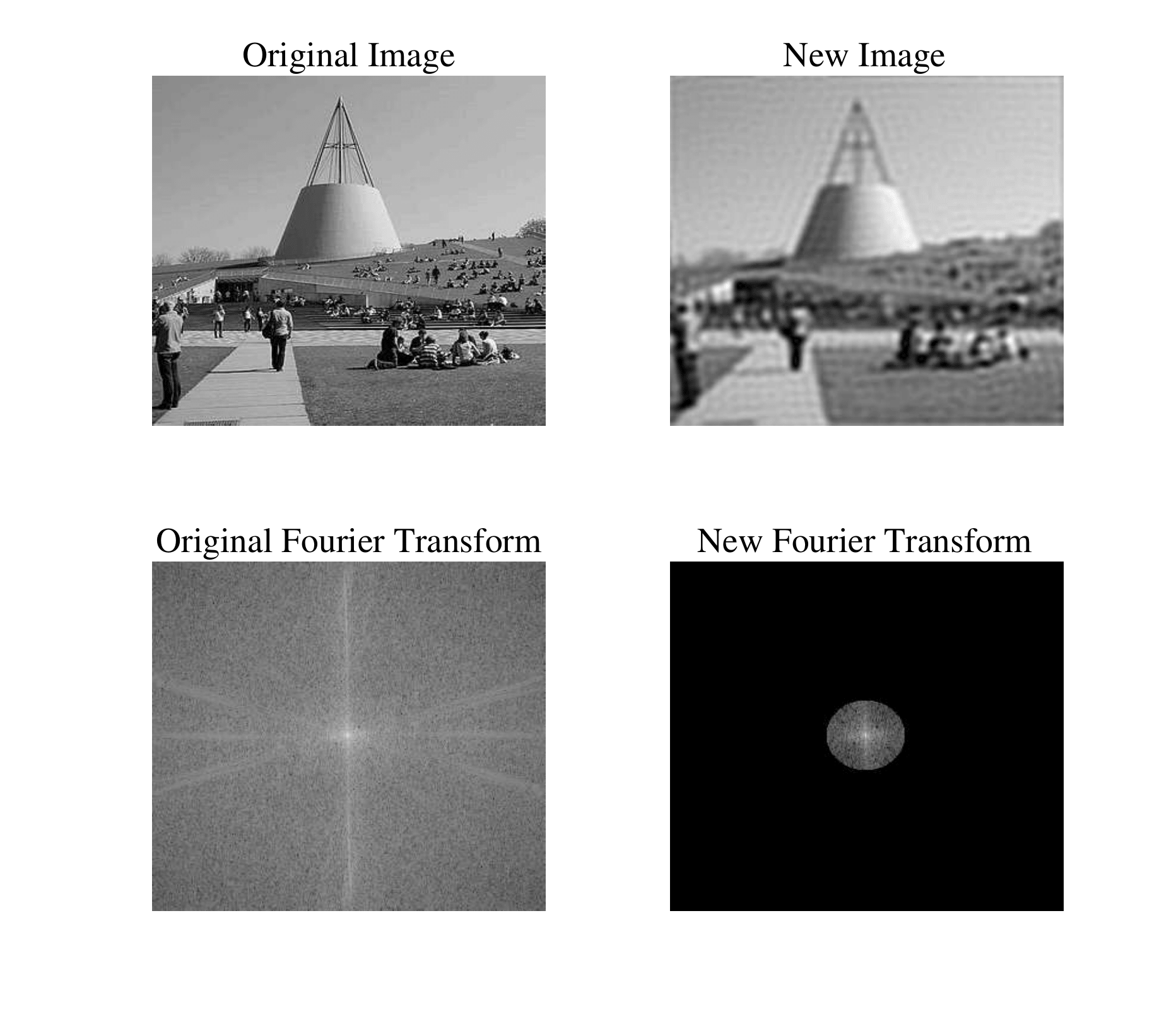
(a) Removing the high spatial frequencies
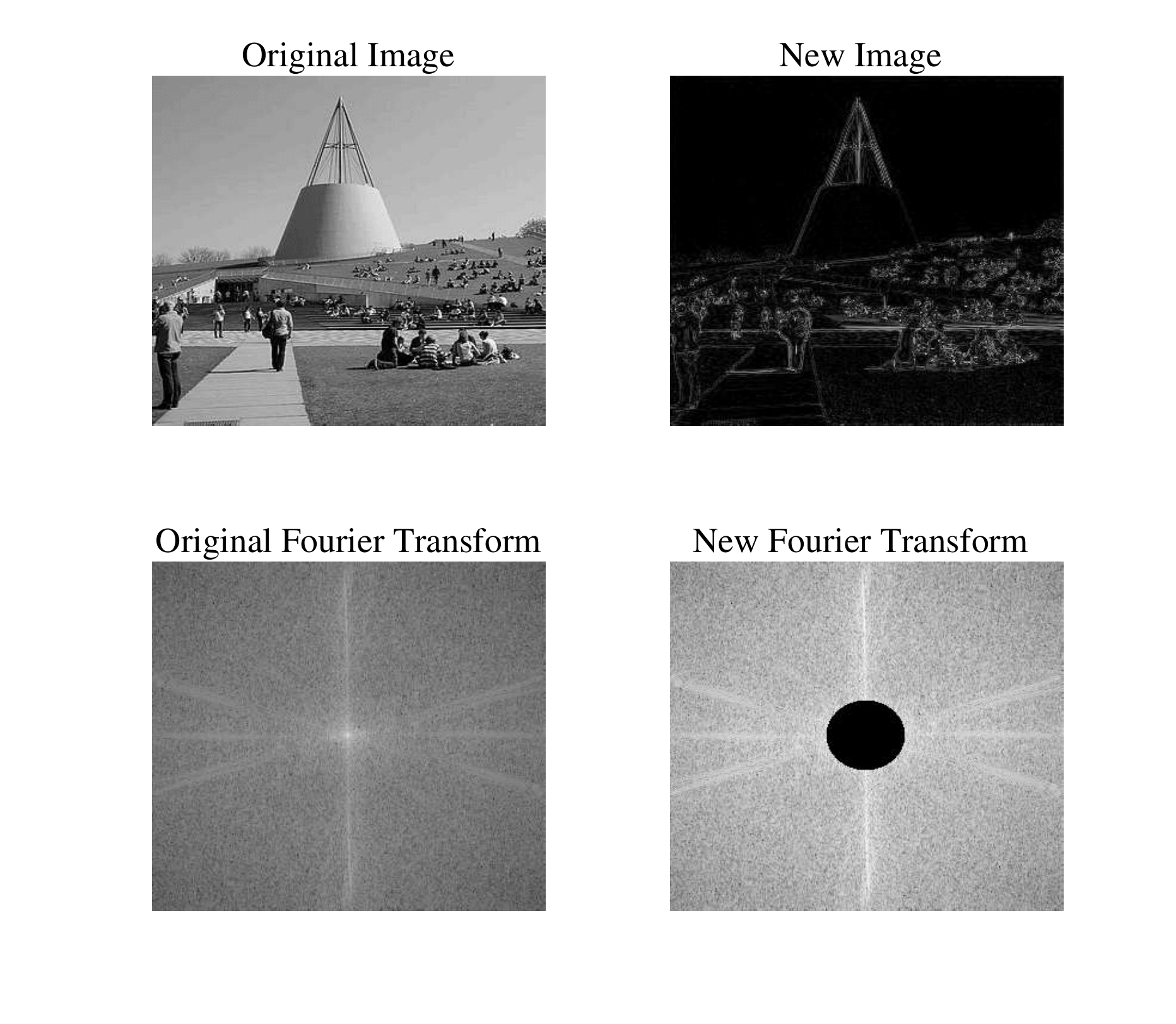
Figure 6:(b) Removing the low spatial frequencies
Demonstration of the roles of different spatial frequencies. By removing the high spatial frequencies, only the broad features of the image remain and resolution is lost. If the low spatial frequencies are removed, only the sharp features (i.e. the contours) remain.
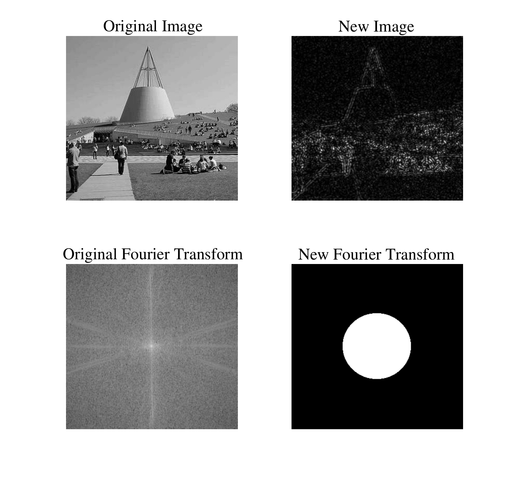
(a) Removing the amplitude information by setting the amplitude of propagating and evanescent waves to 1 and 0, respectively.
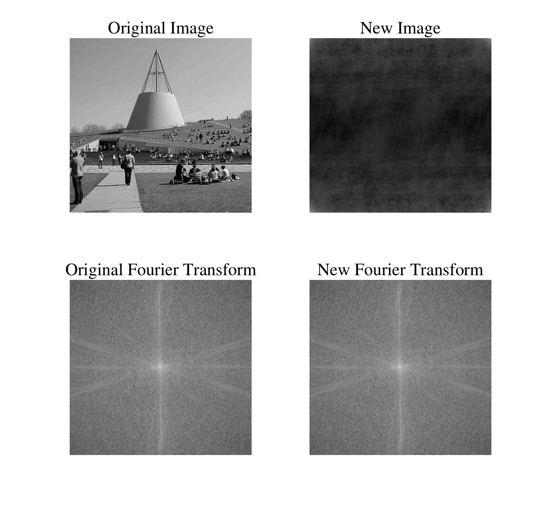
Figure 8:(b) Removing the phase information by setting the phase equal to 0.
Demonstration of the role of the phase of the spatial Fourier transform. If the amplitude information is removed, but phase information is kept, some features of the original image are still recognizable. Removing Fourier phase destroys most recognizable structure in this example; magnitude-only measurements require additional constraints to recover an image.
Another aspect of the Fourier transform is the uncertainty principle. It states that many waves of different frequencies have to be added to get a function that is confined to a small space[4]. Stated differently, if is confined to a very small region, then must be very spread out. This can also be illustrated by the scaling property of the Fourier transform:
which simply states that the more is squeezed by increasing , the more its Fourier transform spreads out. This principle is illustrated in Figure 9. The uncertainty principle is familiar from quantum physics where it is stated that a particle cannot have both a definite momentum and a definite position. In fact, this is just one particular manifestation of the uncertainty principle just described. A quantum state can be described in the position basis as well as in the momentum basis . Up to normalization and the change of variable , the basis transformation between these representations is a Fourier transform
Hence, the two are obviously subject to the uncertainty principle! In fact, any two quantum observables which are related by a Fourier transform (also called conjugate variables), such as position and momentum, obey this uncertainty relation. The uncertainty relation states:
After substantial propagation, the detectable spectrum is effectively limited to propagating transverse wave numbers . A conventional focused field therefore has a characteristic transverse scale of order , with an exact spot size set by its aperture and by the chosen width criterion.
This sets the scale of the conventional far-field diffraction limit.
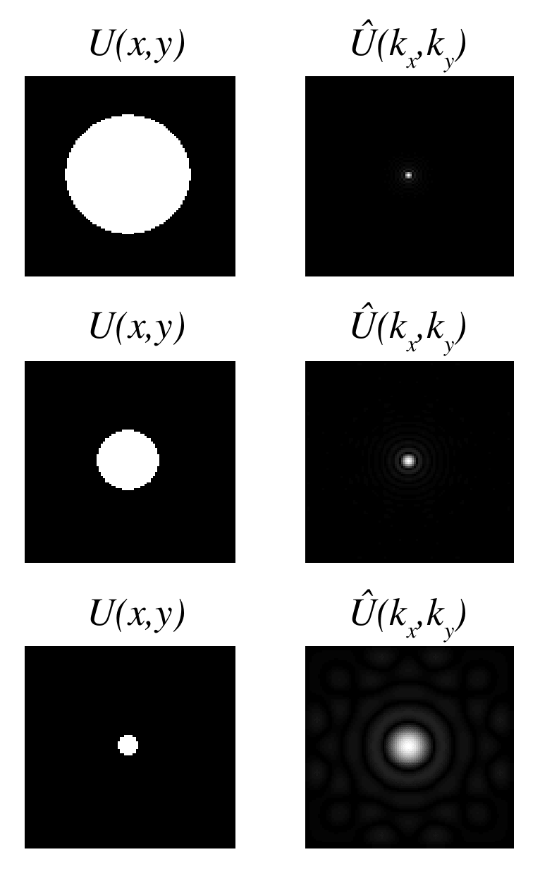
Figure 9:Demonstration of the uncertainty principle. The more confined is, the larger the spread of .
4Fresnel and Fraunhofer Approximations¶
The Fresnel and Fraunhofer approximations are two approximations of the Rayleigh-Sommerfeld integral Eq. (12). The approximations are accurate provided the propagation distance is sufficiently large. In the Fraunhofer approximation, has to be quite large, i.e. larger than for the Fresnel approximation, which is already accurate for typical distances occurring in optical systems. Putting it differently: in order of most accurate to least accurate (i.e. only valid for large propagation distances), the diffraction integrals would rank as:
4.1Fresnel Approximation¶
We assume that in Eq. (12) is so large that in the denominator we can approximate by :
The reason why we cannot apply the same approximation for in the exponent is that in the exponent is multiplied by , which is a very large number at optical frequencies, so any error introduced by approximating would be drastically magnified by multiplying by which can easily lead to a completely different value of . To approximate in we must be more careful and apply a Taylor expansion. Recall that
We know that the Taylor expansion around implies:
Since we assume that is large, is small, so we have
With this approximation, we arrive at the Fresnel diffraction integral, which can be written in the following equivalent forms:
Especially the last expression is interesting, because it shows that
Note that this propagator depends on the distance of propagation .
Remark. By Fourier transforming Eq. (20), one can get the plane wave amplitudes of the Fresnel approximation. It turns out that these amplitudes are equal to multiplied by a phase factor which is obtained from a paraxial approximation of the exact phase factor , i.e. is approximated by a quadratic function of . Therefore the Fresnel approximation is also called the paraxial approximation. In fact, it can be shown that the Fresnel diffraction integral is a solution of the paraxial wave equation and conversely, that every solution of the paraxial wave equation can be written as a Fresnel diffraction integral[5].
4.2Fraunhofer Approximation¶
To obtain the Fraunhofer approximation, we will make one further approximation to in in addition to the Fresnel approximation:
Hence we have omitted the quadratic terms , and in comparison with the Fresnel diffraction integral, we omit the factor to obtain the Fraunhofer diffraction integral:
This leads to the following important observation:
Note that to obtain the Fraunhofer field in , the Fourier transform has to be evaluated at spatial frequencies and . These spatial frequencies scale with and the overall field is proportional to . This implies that when is increased the field pattern spreads out without changing its shape while its amplitude goes down so that the total energy is preserved. Stated differently, apart from the factor in front of the integral, the Fraunhofer field depends on the angles and . Therefore for large propagation distances for which the Fraunhofer approximation is accurate, the field becomes broader (it diverges) when the propagation distance increases.
Remarks.
The Fresnel approximation is, like the Fraunhofer approximation, a Fourier transform of the field in the starting plane (), evaluated at spatial frequencies which depend on the point of observation:
However, in contrast to the Fraunhofer approximation, the Fresnel approximation depends additionally in a different way on the propagation distance , namely through the exponent of the Fresnel propagator in the integrand. Therefore the Fresnel approximation gives quite diverse patterns depending on the propagation distance , as is shown in Figure 12.
In the Rayleigh-Sommerfeld diffraction integral, the field is written as a superposition of spherical waves. In the Fresnel approximation the spherical waves are approximated by parabolic waves. Finally, in the Fraunhofer approximation the propagation distance is so large that the parabolic waves can be approximated by plane waves.
Let be the function obtained from by translation. From the general property of the Fourier transform:
it follows that when the field is translated, the intensity in the Fraunhofer far field is not changed. In contrast, due to the additional quadratic phase factor in the integrand of the Fresnel integral, the intensity of the Fresnel field in general changes when is translated.
Suppose that is the field immediately behind an aperture with diameter in an opaque screen. It can then be shown that points of observation, for which the Fresnel and Fraunhofer diffraction integrals are sufficiently accurate, satisfy:
The Fresnel number is defined by
A small Fresnel number, such as with this definition of , usually makes the Fraunhofer approximation accurate over paraxial observation angles; larger values call for the Fresnel or exact treatment (see Figure 12). Suppose that and the wavelength is that of green light: . Then the illustrative criterion requires , so a distance above about 20 m is appropriate.
The paraxial Fraunhofer formula used here assumes:
Here and approximate direction angles only in the paraxial regime. A large value of does not imply an evanescent wave; it means this approximation is invalid. For example, keeping both ratios below about 0.3 limits the angular error.
In any expression for an optical field, one may always omit factors of constant phase, i.e. an overall phase which does not depend on position. If one is only interested in the field in certain planes , then a factor like may also be omitted. Further, in some cases also a position dependent phase factor in front of the Fresnel and Fraunhofer diffraction integrals is omitted, namely when only the intensity is of interest. In exercises it is usually mentioned that this factor may be omitted: if this is not stated, it should be retained in the formulae.
4.3Examples of Fresnel and Fraunhofer approximations¶
Fresnel approximation of the field of two point sources.
Consider two mutually coherent time-harmonic point sources at and . The fields in emitted are according to the time-harmonic field equation (see the Interference chapter) proportional to
We apply the Fresnel approximation for large :
Hence,
where in the denominator we replaced by . Note that the Fraunhofer approximation amounts to while the phase factor remains. The intensity on a screen of the sum of the two fields for the case that the sources have equal strength and emit in phase is:
In the far field, the intensity results from interference of two approximately plane waves with phase factors and is given by a cosine function (see Figure 10). For these symmetric, equal-amplitude point sources, the common quadratic source phase cancels from the intensity, so the Fresnel and Fraunhofer expressions agree within their shared paraxial range. For more sources at different positions, the Fresnel phases need not be common. The leading paraxial intensity is independent of . Formally, its minima satisfy
and its maxima satisfy
for integers within the valid small-angle range. If , the first formal minimum lies outside that range and no true far-field zero is accessible. The figure below also includes the near field, where these far-field formulas do not apply.
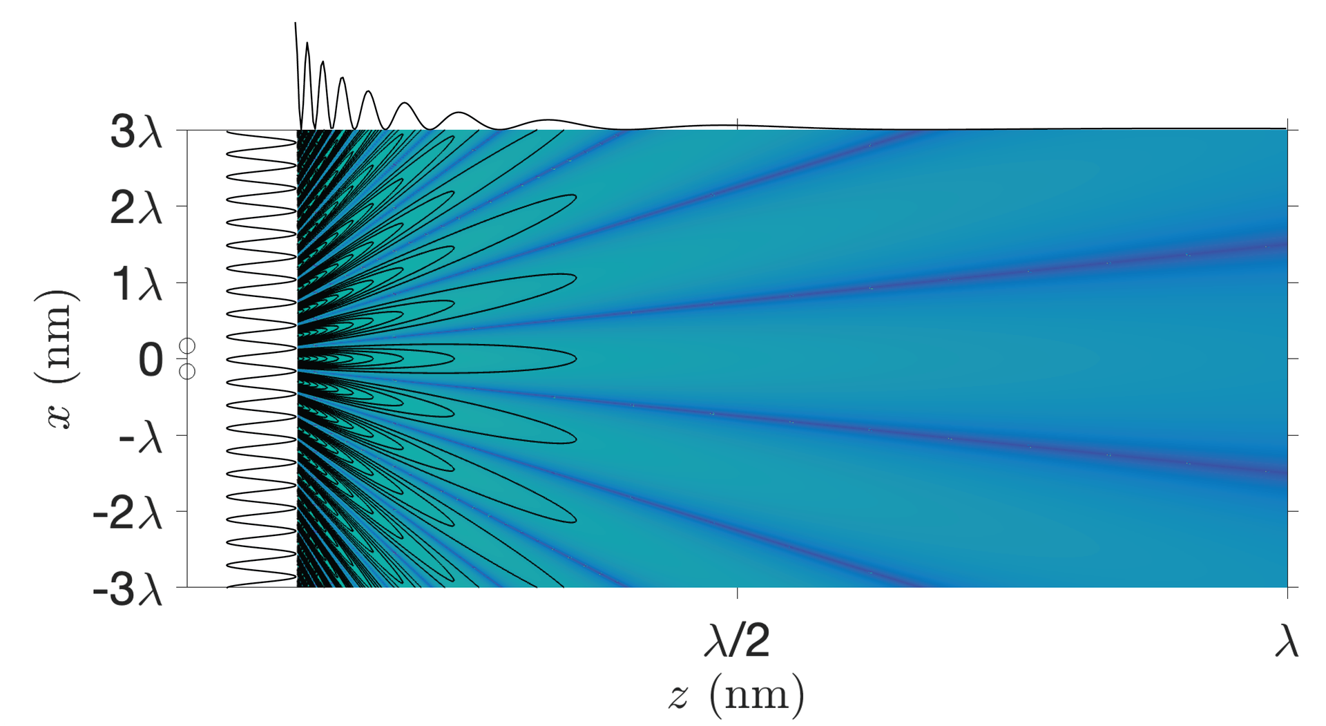
Figure 10:Near-field intensity from two mutually coherent point sources of equal strength and phase at nm. The far-field trend follows Eq. (33). Their separation is 200 nm. The image shows distances of only a few wavelengths and therefore is not a Fraunhofer-pattern example.
Fraunhofer approximation of a rectangular aperture in a screen.
Let the screen be and the aperture be given by , . The transmission function is:
where
and similarly for . Let the aperture be illuminated by a perpendicular incident plane wave with unit amplitude. Then the field immediately behind the screen is:
We have
where . Hence,
The Fraunhofer far field at a large distance from a rectangular aperture in a mask is obtained by substituting Eq. (40) into Eq. (23).
Remarks.
The first zero along the -direction from the center occurs for
The distance between the first two zeros along the -axis is and is thus larger when the width along the -direction of the aperture is smaller.
The single-slit first zero requires . Thus no angular zero is possible for . A subwavelength aperture still affects the measured far field, but inferring its width becomes sensitive to a model, signal-to-noise ratio, and calibration.
As illustrated in Figure 11, the Fraunhofer diffraction pattern as a function of diffraction angle is narrowest in the direction in which the aperture is widest.
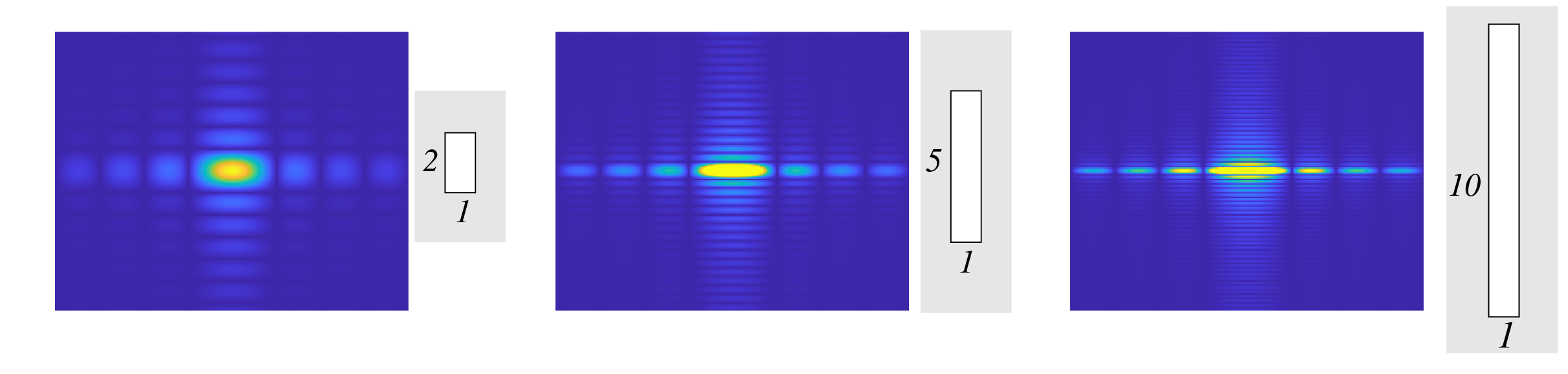
Figure 11:Fraunhofer diffraction pattern of a rectangular aperture in an opaque screen. Left: the width of the aperture in the -direction is twice that in the -direction; middle: the width in the -direction is 5 times that in the -direction; right: the width in the -direction is 10 times that in the -direction.
Fresnel approximation of a rectangular aperture in a mask
The integral in the Fresnel approximation for the field of a rectangular aperture in a mask can be computed analytically and leads to functions that are actually called “Fresnel integrals” which can be studied using the Cornu spirals. We will not go deeper in this matter but simply show the results of the simulations in Figure 12. The distance to the mask increases ( decreases), from very close to the mask at the bottom right, to further from the mask at the bottom left, to rather far from the mask in the upper right, to the Fraunhofer distance in the upper left figures. Note the change in scale along the axis in the figures and the decrease of intensity with propagation distance. It is seen that the pattern changes and broadens drastically with distance from what is more or less a copy of the aperture, to a pattern that is equal to the Fourier transform of the aperture. Once the Fraunhofer approximation is accurate, a further increase of distance only results in a widening of the pattern and a decrease of overall amplitude without change of shape. In contrast, in the region where the Fresnel approximation is accurate, the shape of the pattern is seen to change a lot with distance to the mask.
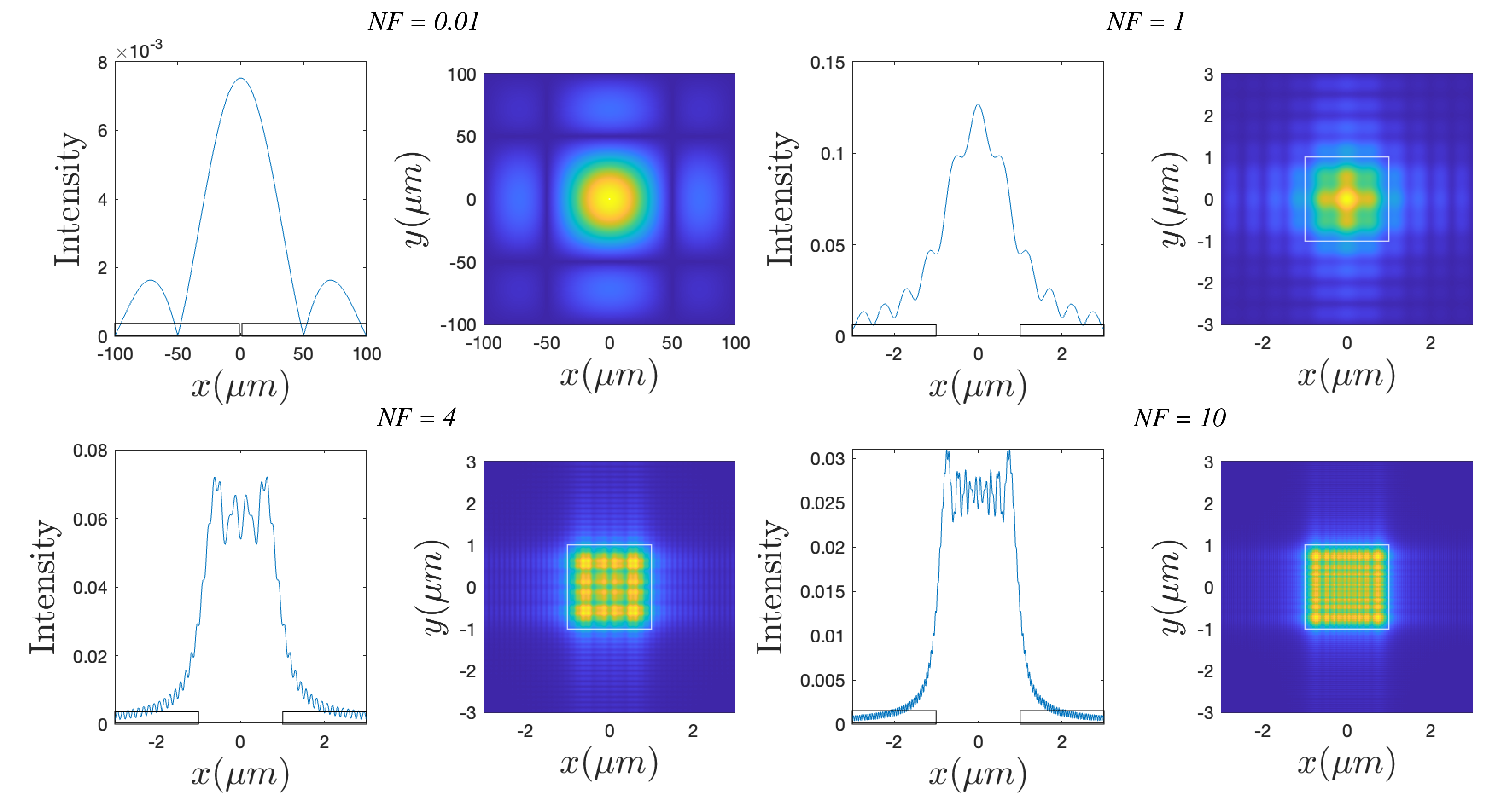
Figure 12:Diffraction patterns of a square opening in a mask with corresponding cross-sections along the -axis, showing the transition from Fresnel to Fraunhofer approximations. The distance to the mask increases as the Fresnel number decreases from the near field pattern close to the mask in the right bottom figures to the Fraunhofer diffraction pattern in the upper left. Note the different scales along the axis in the figures.
Fraunhofer approximation of a periodic array of slits
We can now predict the diffraction pattern of an array of slits of finite width. It follows from the Fraunhofer pattern of a single rectangular aperture that, if the sides parallel to the -direction are very long, the Fraunhofer diffraction pattern as a function of angle in the -direction is very narrow. In Figure 11b the Fraunhofer diffraction pattern of a rectangular aperture is shown, of which the width in the -direction is 10 times the width in the -direction. The diffraction pattern is then strongly concentrated along the -axis. If we only consider the Fraunhofer pattern for while still considering it as a function of , it suffices to compute the Fourier transform only with respect to . The problem then becomes a diffraction problem for a one-dimensional slit.
We consider now an array of such slits of which the long sides are all parallel to the -axis and we neglect from now on the -variable. Suppose is the function that describes the transmission of a single slit. Then the transmission function of equidistant slits is
where is the distance between neighboring slits, i.e. is the period of the row. If the illumination is by a perpendicular incident plane wave with unit amplitude, the transmitted near field is simply . Then
where for a slit with width we have according to Eq. (39):
The condition must hold. Using
we get
The intensity of the Fraunhofer far field is:
where is the small diffraction angle. The factor
oscillates rapidly with because the sine argument in the numerator contains the factor of while is a slowly varying envelope. This is a manifestation of the property of the Fourier transform that small details of a structure (e.g. the size of a single slit) cause large scale features of the far field pattern, whereas large scale properties such as the length of the total structure cause quickly changing features. This is illustrated in Figure 13.
The grating interference factor is maximum for directions where both the denominator and numerator of Eq. (48) vanish:
These directions are called diffraction orders. The exact ray path condition is ; the formulas here use for small angles. At the paraxial order directions,
The sine ratio tends to at an order. Therefore the intensity of the th order is
hence it is proportional to the square of the number of periods and to the squared modulus of the envelope in .
Between two adjacent diffraction orders, Eq. (48) has zeros and secondary maxima (see Figure 13). The angular width of a diffraction order is half the angular distance to the nearest zeros next to the order, i.e.
If there are more slits, the intensity peaks into which the energy is diffracted are narrower and the peaks are higher.
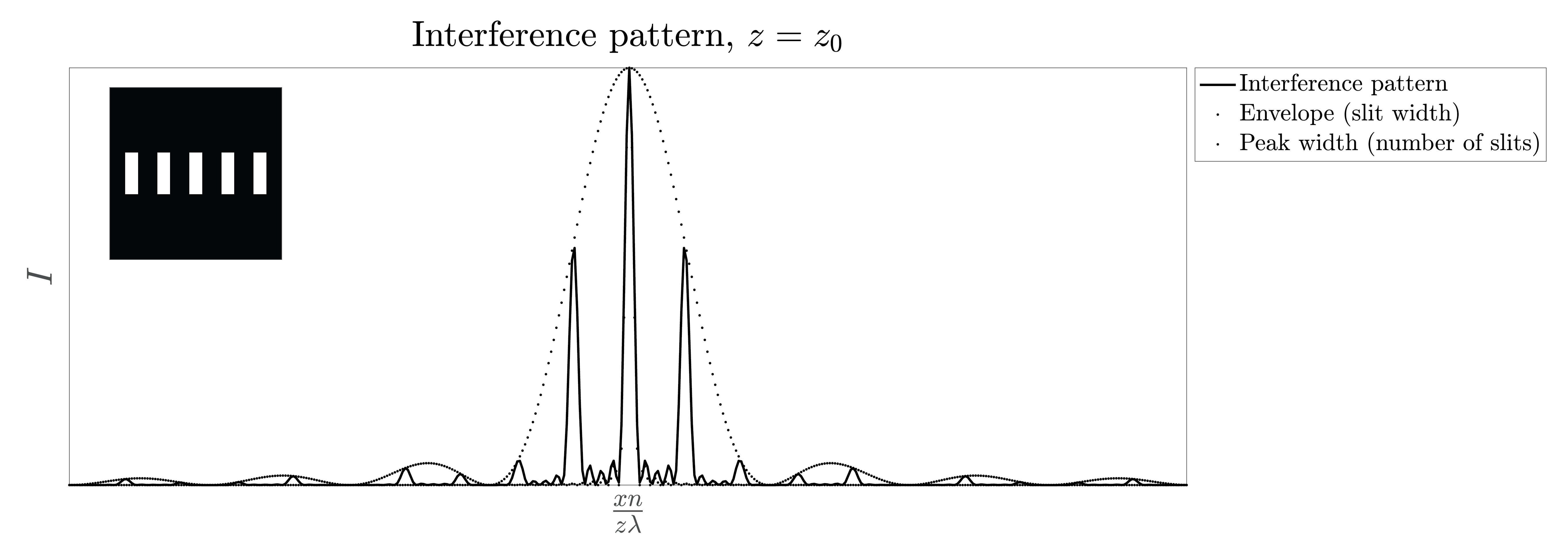
Figure 13:An illustration of a diffraction pattern of a series of five slits.
The exact grating condition requires . This limits the propagating orders:
Hence, the larger the ratio of the period to the wavelength, the more diffraction orders.
The property Eq. (49) that the diffraction orders depend on wavelength is used to separate wavelengths. Grating spectrometers use periodic structures such as an array of slits to very accurately separate and measure wavelengths. The th diffraction orders of two wavelengths and are just separated if
which implies with and that
It follows that the resolution is higher when there are more slits and for a larger diffraction order. However, the disadvantage of using higher diffraction orders is that often their intensity is less. For a grating with 1000 periods one can obtain a resolution of in the first order.
It should be remarked that a grating is obtained for any periodic variation of the refractive index. If the proper transmission function for the unit cell of the grating is substituted for , the formulae above also give the Fraunhofer far field of such more general diffraction gratings. By changing the unit cell, the envelope of the diffraction pattern can be changed and a certain order can be given more intensity. In Figure 14 a so-called blazed grating is shown which is used in reflection and which has a strong first diffracted order for a certain angle of incidence.
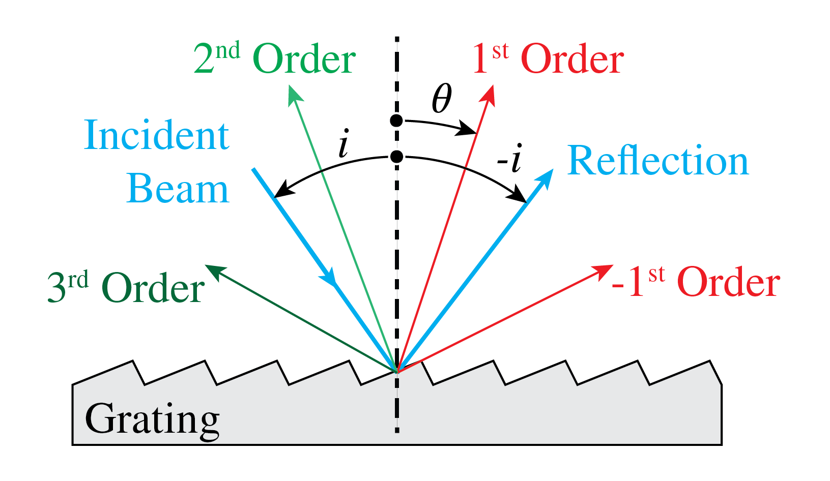
Figure 14:Diffraction grating used in reflection with a so-called blazed unit cell.
Remark. A periodic row of slits is an example of a diffraction grating. A grating is a periodic structure, i.e. the refractive index is a periodic function of position. Structures can be periodic in one, two and three directions. A crystal acts as a three-dimensional grating whose period is the period of the crystal, which typically is a few Angstroms. X-rays have wavelengths comparable to atomic spacings, ranging across and below the ångström scale. When a beam of x-rays illuminates a crystal, a detector in the far field measures the Fraunhofer diffraction pattern given by the intensity of the Fourier transform of the refracted near field. These diffraction orders of crystals for x-rays were discovered by Von Laue and are used to study the atomic structure of crystals.
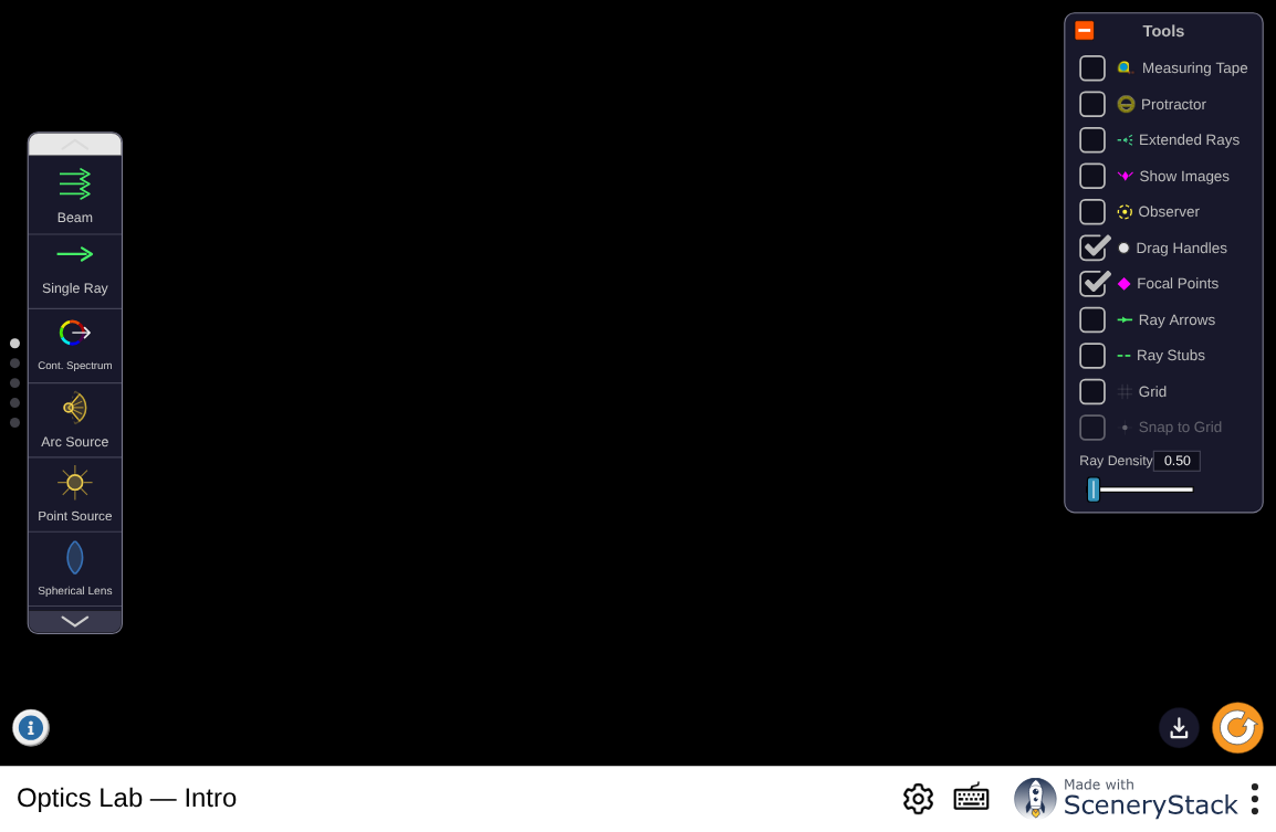
Figure 15:Transmission and reflection gratings on an optical bench. Change the grating period and the illuminating wavelength and watch the diffracted orders move — a geometric-optics preview of the far-field grating condition used for crystals and for laboratory diffraction gratings.
Interactive simulation: Optics Lab
5Fraunhofer Diffraction Revisited¶
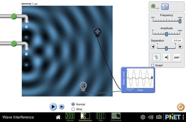
Figure 16:An aperture and the far-field pattern it produces, with size, shape, and wavelength adjustable. Everything narrow in the aperture is wide in the pattern — the scaling of Fraunhofer diffraction, seen whole rather than one angle at a time.
Interactive simulation: Wave Interference
Fraunhofer diffraction patterns can qualitatively be explained by considering directions in which destructive and constructive interference occur. Consider two mutually coherent point sources , on the -axis as shown in Figure 17. We assume that these point sources are in phase. On a screen at large distance an interference pattern is observed. If the distance of the screen is very large, the spherical wave fronts emitted by the point sources are almost plane at the screen and the field is the Fraunhofer far field of the two point sources. At point on the screen at a distance above the -axis the optical path difference of the waves emitted by the two sources is approximately given by , where is assumed small. Hence constructive interference occurs for angles such that for some integer , i.e. when
Destructive interference occurs when the path length difference satisfies for some integer , hence for angles
If the point sources have the same strength, their fields perfectly cancel for these angles.
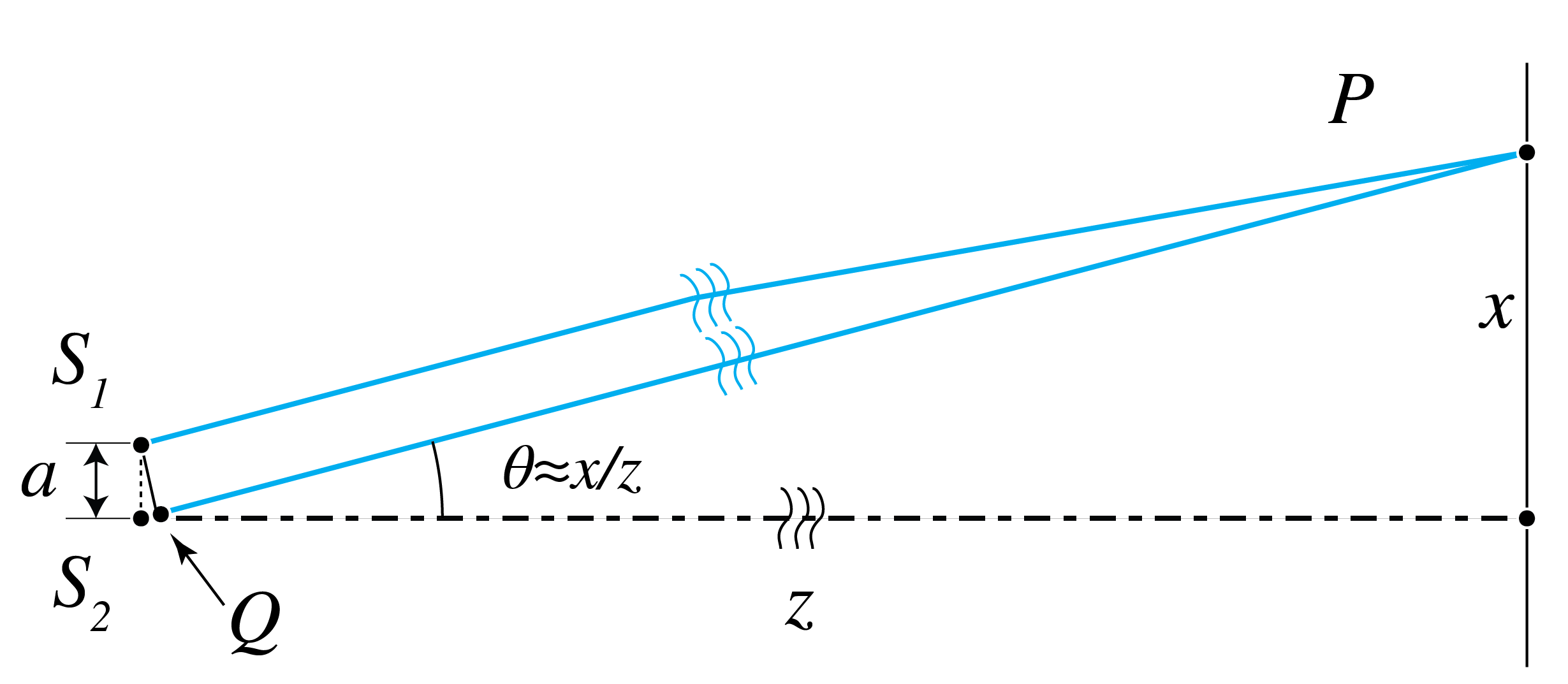
Figure 17:Interference of two mutually coherent point sources. For very large , points where constructive or destructive interference occurs satisfy for some integer : and , respectively.
Now consider a slit as shown in Figure 18 which is illuminated by a perpendicular incident plane wave. By the Huygens-Fresnel principle, the field at a screen far from the slit is the sum of the fields of point sources in the aperture, with strengths proportional to the field in the slit at the position of the point sources. When the slit is illuminated by a plane wave at perpendicular incidence, all point sources are in phase and have equal strength. Divide the slit into two equal halves as shown in Figure 18. The point sources in the slit can be arranged into pairs, of which one point source is in the upper half of the slit and the other is at the equivalent position (at distance from the other point source) in the lower half of the slit. Let be an angle for which the two point sources of a pair cancel each other i.e.
since the distance between the point sources is . By translating the pair of point sources through the slit, it follows that both half slits perfectly cancel each other for these angles. In this way we have found the angles with odd for which destructive interference occurs. Destructive interference for even can be derived by further subdivisions of the aperture.
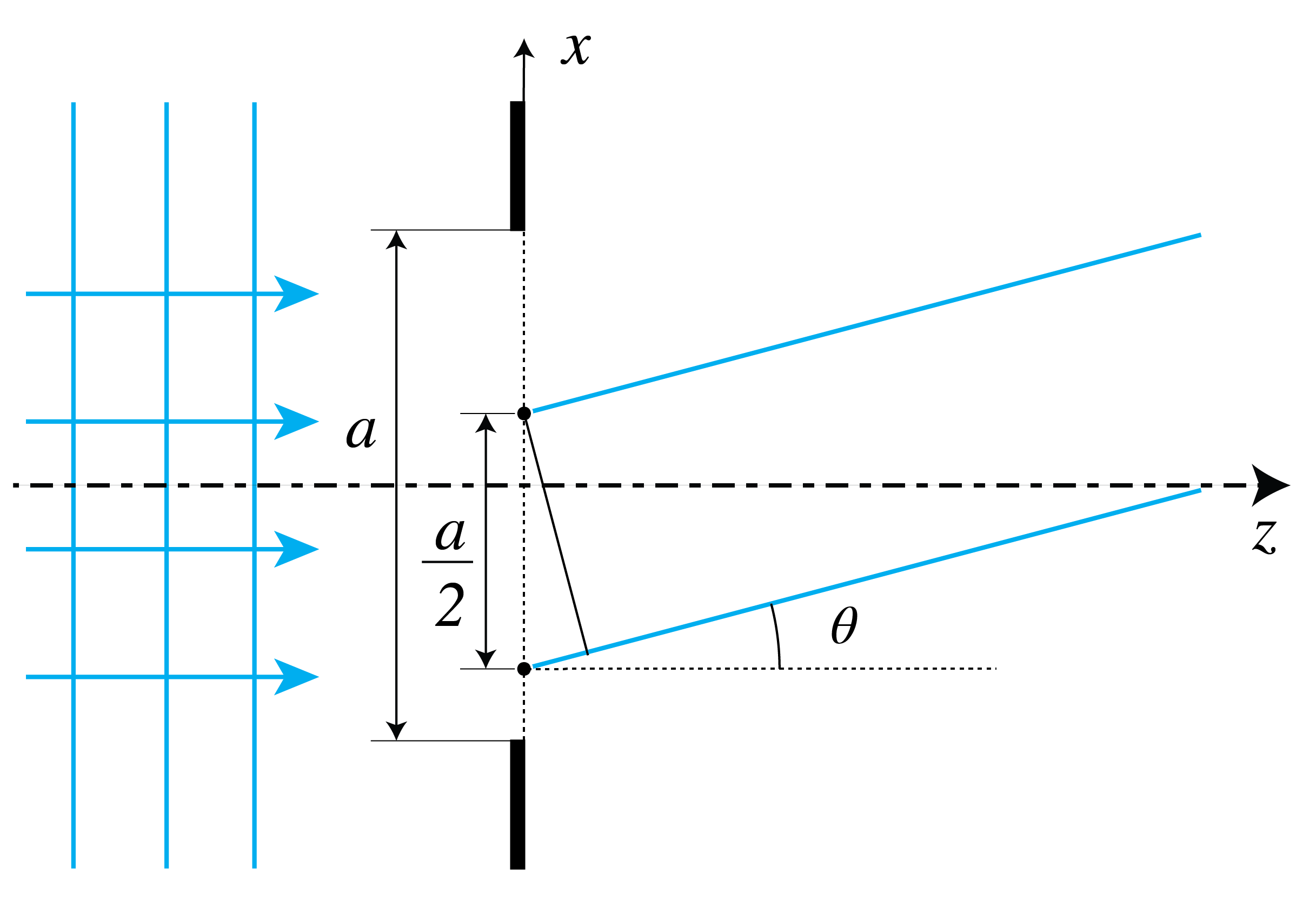
Figure 18:By dividing the slit into two slits of size each and considering pairs of point sources of which one is in the upper half of the slit and the other is at the corresponding position in the lower half, angles where destructive interference occurs between these point sources lead to minima in the diffraction pattern. Note that the point sources have corresponding positions in the two parts of the slit if their distance is .
In general it is easier to find the angles for which the far field vanishes than to find (local) maxima of the field. An exception is the case of a diffraction grating. It follows from Figure 19 that there will be constructive interference between adjacent periods, and hence for all periods, for angles for which the distance in Figure 19 is a multiple of the wavelength, i.e. for
which corresponds to the direction of the diffraction orders. For other angles the phases of the fields of the different periods differ widely and therefore the fields almost cancel at these angles when there are many periods. This explains that for a diffraction grating of many periods, the far field intensity is highly concentrated in particular directions given by the orders Eq. (59) which depend only on the ratio of the wavelength and the period.
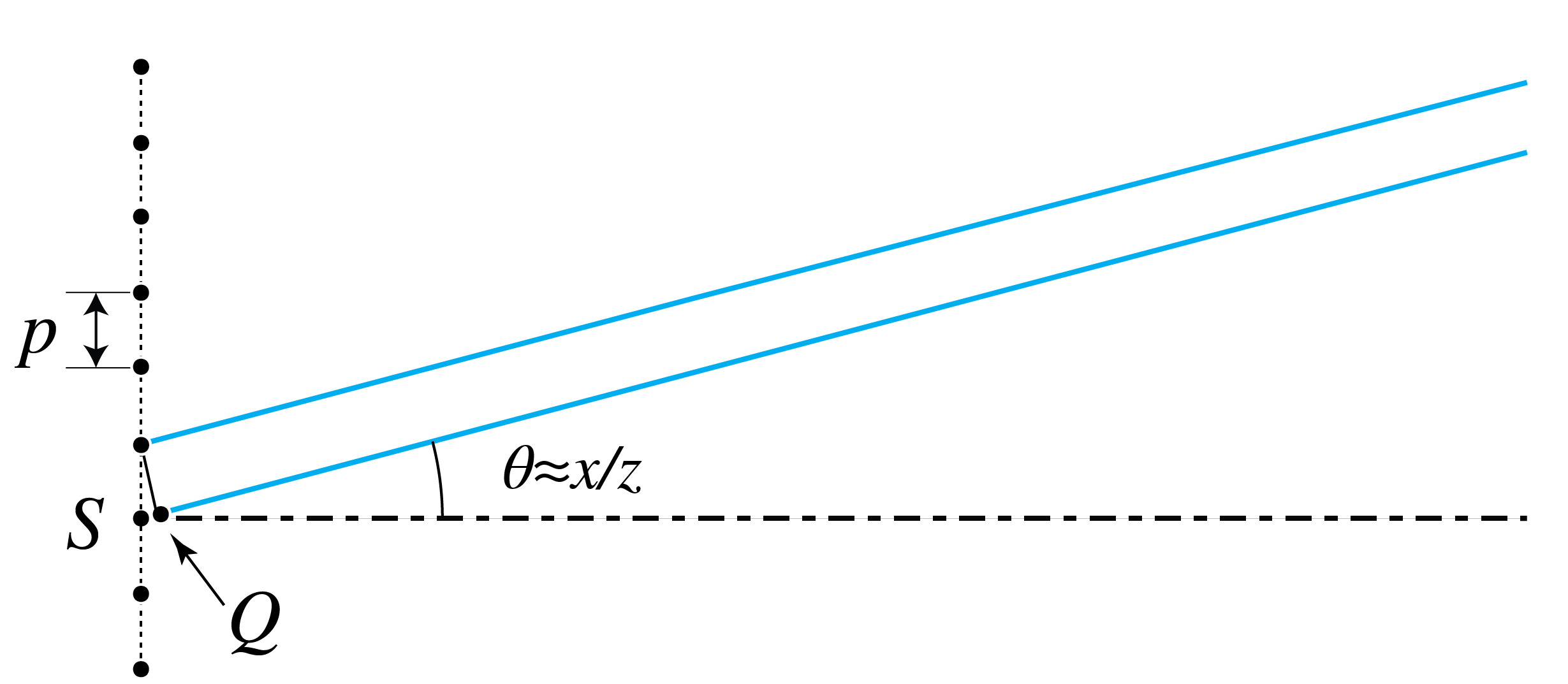
Figure 19:If the angle is such that is a multiple of the wavelength, two adjacent periods, and hence all periods of the grating, constructively interfere. These angles correspond to the diffraction orders.
6Fourier Optics¶
In this section we apply diffraction theory to a lens. We consider in particular the focusing of a parallel beam and the imaging of an object.
6.1Focusing of a Parallel Beam¶
A lens induces a local phase change to an incident field in proportion to the local thickness of the lens. Let a plane wave which propagates parallel to the optical axis be incident on a positive lens. In Gaussian geometrical optics the incident rays are all focused into the image focal point. According to the Principle of Fermat, all rays have traveled the same optical distance when they intersect in the image focal point where they constructively interfere and cause an intensity maximum. In the focal region, the wavefronts are parts of spheres centered at the focal point and cut off by the cone with the focal point as top and opening angle , as shown in Figure 20. Behind the focal point, there is a second cone with again spherical wavefronts, but there the light is propagating away from the focal point. According to Gaussian geometrical optics, image space is completely dark outside the two cones in Figure 20. However, as we will show, in diffraction optics this is not true.
We assume that the lens is thin and choose as origin of the coordinate system the center of the thin lens with the positive -axis along the optical axis. Let be the -coordinate of the image focal point according to Gaussian geometrical optics. Then is the image focal point. Let be a point between the lens and this focal point. According to geometrical optics the field in is proportional to
where we have included the time-dependence. Indeed the surfaces of constant phase:
are spheres centered at the focal point. For increasing time, these spheres converge to the focal point, while the amplitude increases as the distance to the focal point decreases, so that energy is preserved.
Remark. For a point to the right of the focal point, i.e. for , the spherical wave fronts propagate away from the focal point and therefore there should be replaced by in the exponent in Eq. (60).
The exit pupil of the lens is in the plane where, according to Eq. (60), the field is
where the time dependence has been omitted and
i.e. for in the exit pupil of the lens and otherwise. If is sufficiently small, we may replace the distance between a point in the exit pupil and the image focal point in the denominator of Eq. (62) by . This is not allowed in the exponent, however, because of the multiplication by the large wave number . In the exponent we therefore use instead the first two terms of the Taylor series Eq. (18):
which is valid for sufficiently small. Then Eq. (62) becomes:
where we dropped the constant factors and . For a general field incident on the lens, i.e. in the entrance pupil, the lens applies a transformation such that the field in the exit plane becomes:
The function that multiplies is the transmission function of the lens:
This result makes sense: in the center the lens is thickest, so the phase is shifted the most (but we can define this phase shift to be zero because only phase differences matter, not absolute phase). As is indicated by the minus-sign in the exponent, the further you move away from the center of the lens, the less the phase is shifted. For shorter , the lens focuses more strongly, so the phase shift changes more rapidly as a function of the radial coordinate. Note that the transmission function Eq. (67) has modulus 1 so that energy is conserved.
The field on the right-hand side of Eq. (66) is used in diffraction optics as the field in the exit pupil. But instead of using ray tracing, the field in the focal region is computed using diffraction integrals. We substitute the field in the exit pupil in the Fresnel diffraction integral Eq. (20) and obtain:
The intensity is shown at the bottom left of Figure 20. It is seen that the intensity does not monotonically increase for decreasing distance to the focal point. Instead, secondary maxima occur along the optical axis. Also the boundary of the light cone is not sharp, as predicted by geometrical optics, but diffuse. The bottom right of Figure 20 shows the phase in the focal region. The wave fronts are close to but not exactly spherical inside the cones.
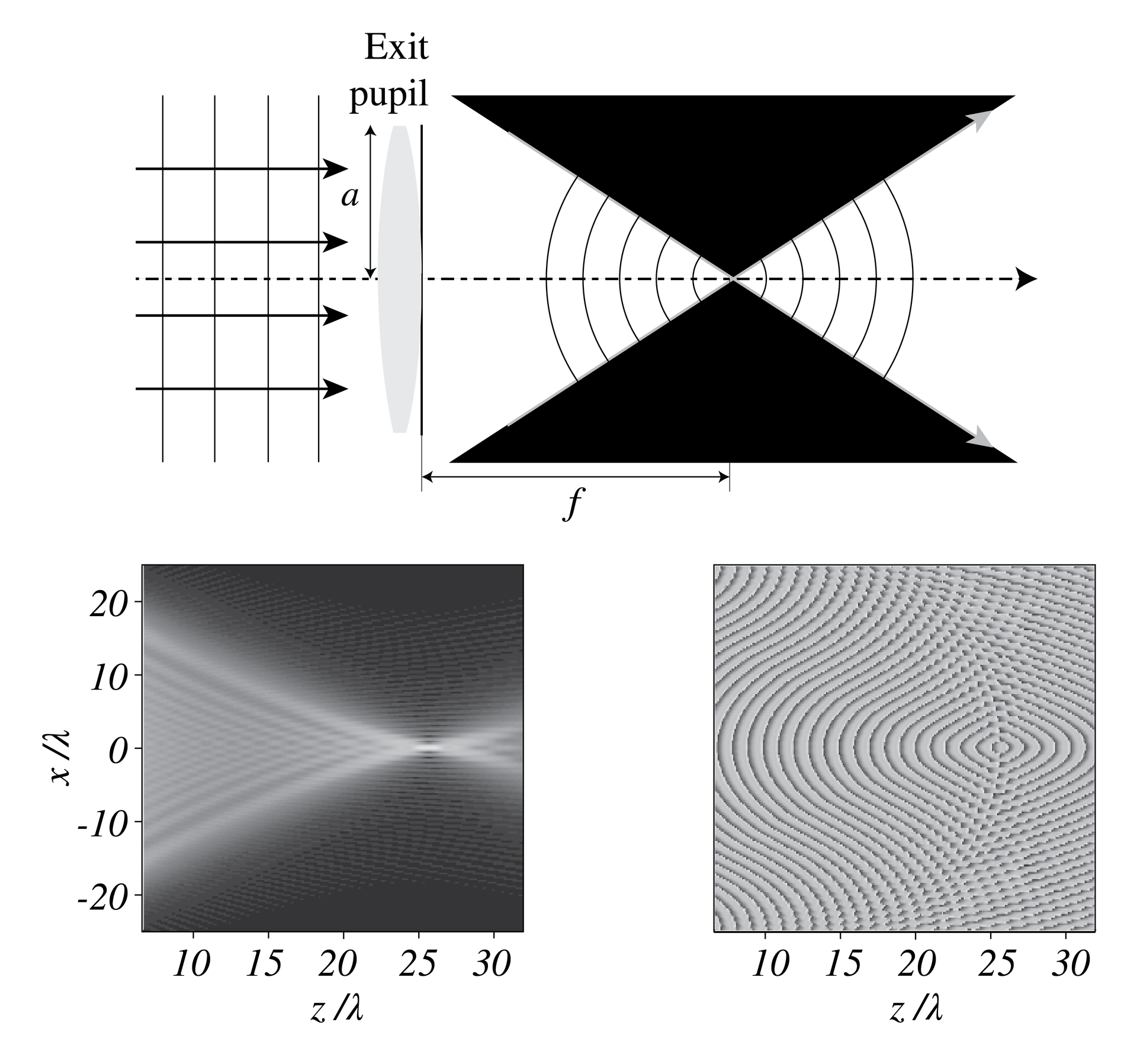
Figure 20:Top: wavefronts of the incident plane wave and the focused field according to Gaussian geometrical optics. There is no light outside of the two cones. Bottom left: amplitude as predicted by diffraction optics. The boundary of the cones is diffuse and it is not absolutely dark outside of the cones. Furthermore, the intensity does not increase monotonically with decreasing distance to the focal point, as predicted by geometrical optics. Bottom right: phase of the focused field as predicted by diffraction optics.
For points in the image focal plane of the lens, i.e. , we have
which is the same as the Fraunhofer integral for propagation over the distance !
It can be shown that the fields in the front focal plane and the back focal plane are related exactly by a Fourier transform, i.e. without the quadratic phase factor[6]. So a lens performs a Fourier transform. Let us see if that agrees with some of the facts we know from geometrical optics.
We know from Gaussian geometrical optics that if we illuminate a positive lens with rays parallel to the optical axis, these rays all intersect in the image focal point. This corresponds with the fact that for (i.e. plane wave illumination, neglecting the finite aperture of the lens, i.e. neglecting diffraction due to the finite size of the pupil), the Fourier transform of the pupil field is a delta peak:
which represents the perfect focused spot (without diffraction).
If in Gaussian geometrical optics we illuminate a lens with tilted parallel rays of light (a plane wave propagating in an oblique direction), then the point in the back focal plane where the rays intersect is laterally displaced. A tilted plane wave is described by , and its Fourier transform with respect to is given by
which is indeed a shifted delta peak (i.e. a shifted focal spot).
It seems that the diffraction model of light confirms what we know from geometrical optics. But in the previous two examples we discarded the influence of the finite size of the pupil, i.e. we have left out of consideration the function in calculating the Fourier transform. If in the entrance pupil and we take the finite size of the pupil properly into account, the -peaks become blurred: the focused field is then given by the Fourier transform of the circular disc with radius , evaluated at spatial frequencies , . This field is called the Airy spot and is given by Eq. (72):
where is the Bessel function of the first kind and where the phase factors in front of the Fourier transform have been omitted. The pattern is shown in Figure 21. It is circularly symmetric and consists of a central maximum surrounded by concentric rings of alternating zeros and secondary maxima with decreasing amplitudes. In cross-section, as a function of , the Airy pattern is similar (but not identical) to the -function. From the uncertainty principle illustrated in Figure 9 it follows that the size of the focal spot decreases as increases, and from Eq. (72) we see that the Airy function is a function of the dimensionless variable . Hence the focal spot becomes narrower as increases. For this paraxial lens in air, its numerical aperture is approximately
Since the first zero of the Airy pattern occurs at , its first-zero radius in this paraxial air-space model is
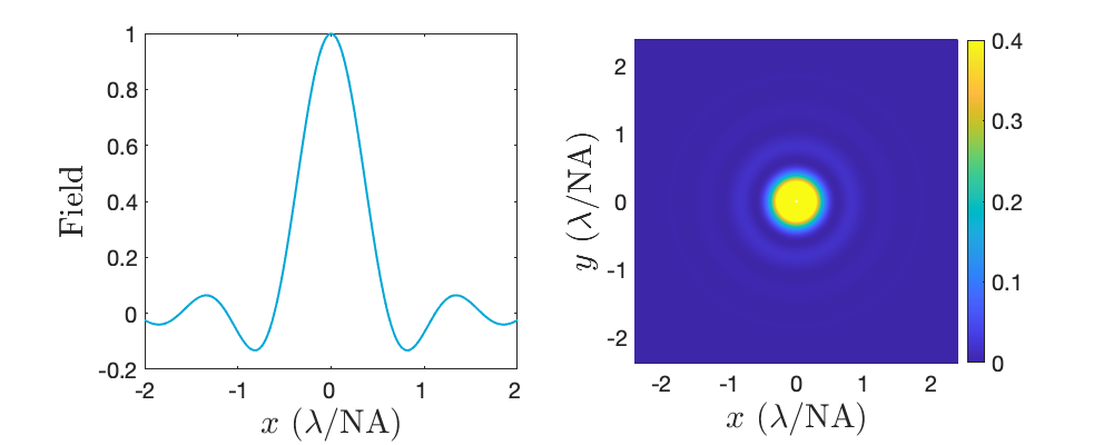
Figure 21:Left: cross section of the field of the Airy pattern. Right: intensity of the Airy pattern.
Remark. In the simple case of a single thin lens, the entrance and exit pupils coincide with the lens itself. As has been explained in the Stops section of the Geometrical Optics chapter, the exit pupil in systems consisting of several lenses is the real or virtual image of the aperture stop under all optical lenses to the right of the stop. To model the effect of diffraction in such more complicated systems, diffraction is assumed to take place entirely in the exit pupil. The field in the exit pupil is first determined by non-paraxial ray tracing and is then integrated over the exit pupil using the Fresnel diffraction integral.
6.2Imaging by a lens¶
It follows from the derivations in the previous section that the Airy pattern is the image of a point source infinitely far in front of a lens. In this section we study the imaging of a general object at a finite distance from the lens. Consider first a real point object on the optical axis with coordinate to the left of the object focal point of a positive lens with image focal coordinate . This lens will form a real image with positive coordinate .
The field in image space is derived using the Fresnel diffraction integral, similar to the focused field in the previous section. We postulate that the lens transforms the field radiated by the point object into a spherical wave in the exit pupil, which converges to the ideal image point of Gaussian geometrical optics. We substitute this spherical pupil field in the Fresnel diffraction integral to compute the field in image space. Then for an object point on the optical axis we find the same Airy pattern as in Figure 21, except that the variable is replaced by , where is the image coordinate found from the lens equation. This field is called the Point Spread Function (PSF):
For object points that are not on the optical axis, the PSF is translated such that it remains centered on the ideal Gaussian image point.
A general object field can be considered a superposition of point objects, and the images of these points are given by translated PSFs:
where are the transverse coordinates of the image point according to Gaussian geometrical optics. The total image field is obtained by summing (integrating) over these PSFs, weighted by the field at the object points:
Here is the signed transverse magnification. An overall scale factor is omitted from the field integral. The integral can be made into a convolution by using the coordinates as integration variables.
It is clear from Eq. (75) that a larger radius of the lens and a smaller wavelength imply a narrower PSF. This in turn implies that the kernel in the convolution is more sharply peaked and hence that the resolution of the image is higher [7].
Remark.
If laser light is used to illuminate the object, the object field may be considered perfectly coherent. This implies that a detector in the image plane would measure the squared modulus of the complex field Eq. (77):
In this case the system is called a coherent imaging system.
If the object is a spatially incoherent extended source, the cross terms between independent source points vanish after averaging. Therefore, in this case the intensity in the image plane is given by the incoherent sum:
where is the mean intensity distribution of the extended source. Hence the image intensity is expressed in terms of the intensity of the source by a convolution with the intensity of the PSF. This system is called an incoherent imaging system.
An object is often illuminated by a spatially incoherent extended light source and then imaged. According to the discussion in the Propagation of Mutual Coherence section of the Interference chapter, the field that illuminates the object is then partially coherent. It is more coherent when the angle that the source extends at the object is smaller. The intensity in the image plane can be computed by splitting the spatially incoherent source into sufficiently many mutually incoherent point sources and computing the intensities in the image plane due to the illumination of the object by each individual point source. The total intensity in the image plane is then the sum of these intensities.
We have considered only scalar diffraction theory. However, for a lens with numerical aperture larger than 0.6, the change of polarization can be important. Then a more general diffraction theory is needed [8].
6.3Spatial Light Modulators and Optical Fourier Filtering¶
SLM. The field in the entrance pupil of a lens, in particular its phase can be changed spatially by a so-called spatial light modulator (SLM). An SLM has thousands of pixels by which very general focused fields can be made. An example is a focused field with only a longitudinal component in the focal point (i.e. only the -component is nonzero at the focal point) [9].
Fourier filtering. Suppose we have the setup as shown in Figure 22. With one lens we can create the Fourier transform of some field . Let a mask be put in the focal plane and a second lens be used to refocus the light. This implies that the amplitude and/or phase of the plane waves in the angular spectrum of the field are manipulated. The procedure is called Fourier filtering using lenses. An application of this idea is the phase contrast microscope.
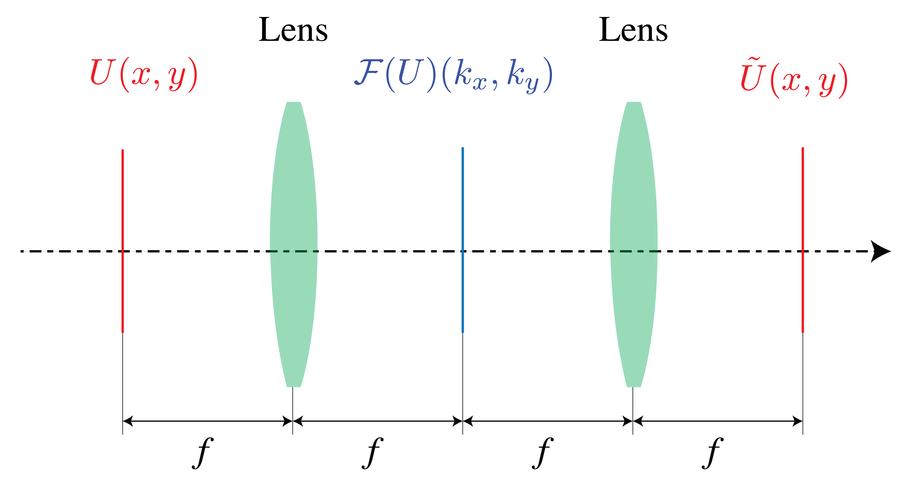
Figure 22:Set-up for Fourier filtering. The first lens creates a Fourier transform of , to which we can apply some operation (e.g. applying different phase shifts to different parts of the field). The second lens then applies another Fourier transform (which gives an inverted image after the second transform, up to scale and phase factors).
7Super-resolution¶
Ordinary far-field imaging is limited by the propagating spatial frequencies admitted by the pupil. Evanescent components decay with distance, and a finite numerical aperture rejects some propagating components as well. The Airy first-zero radius in image space is
For a single thin lens in air, and the object-side numerical aperture is approximately . In a general optical system, entrance and exit pupil sizes must be treated separately. These formulas describe the conventional linear, diffraction-limited image of a point. The examples below gain different kinds of resolution by changing the illumination, detection, medium, or response of the specimen.
Confocal microscopy. A focused spot scans the specimen while a pinhole rejects out-of-focus light before detection. The effective image response is the product of the illumination and detection point-spread functions. This can sharpen the lateral response modestly and improves optical sectioning, at the cost of scanning time. The exact gain depends on pinhole size and illumination and detection wavelengths.
The ideal negative-index slab. Pendry proposed a slab whose permittivity and permeability are the negatives of the surrounding medium. In the ideal model, propagating waves refocus and evanescent components are amplified inside the slab enough to compensate for their decay outside it. This predicts a subwavelength image near the slab. The result relies on exact material matching and arbitrarily large transverse wave numbers; absorption, dispersion, and finite structural scale limit real implementations.
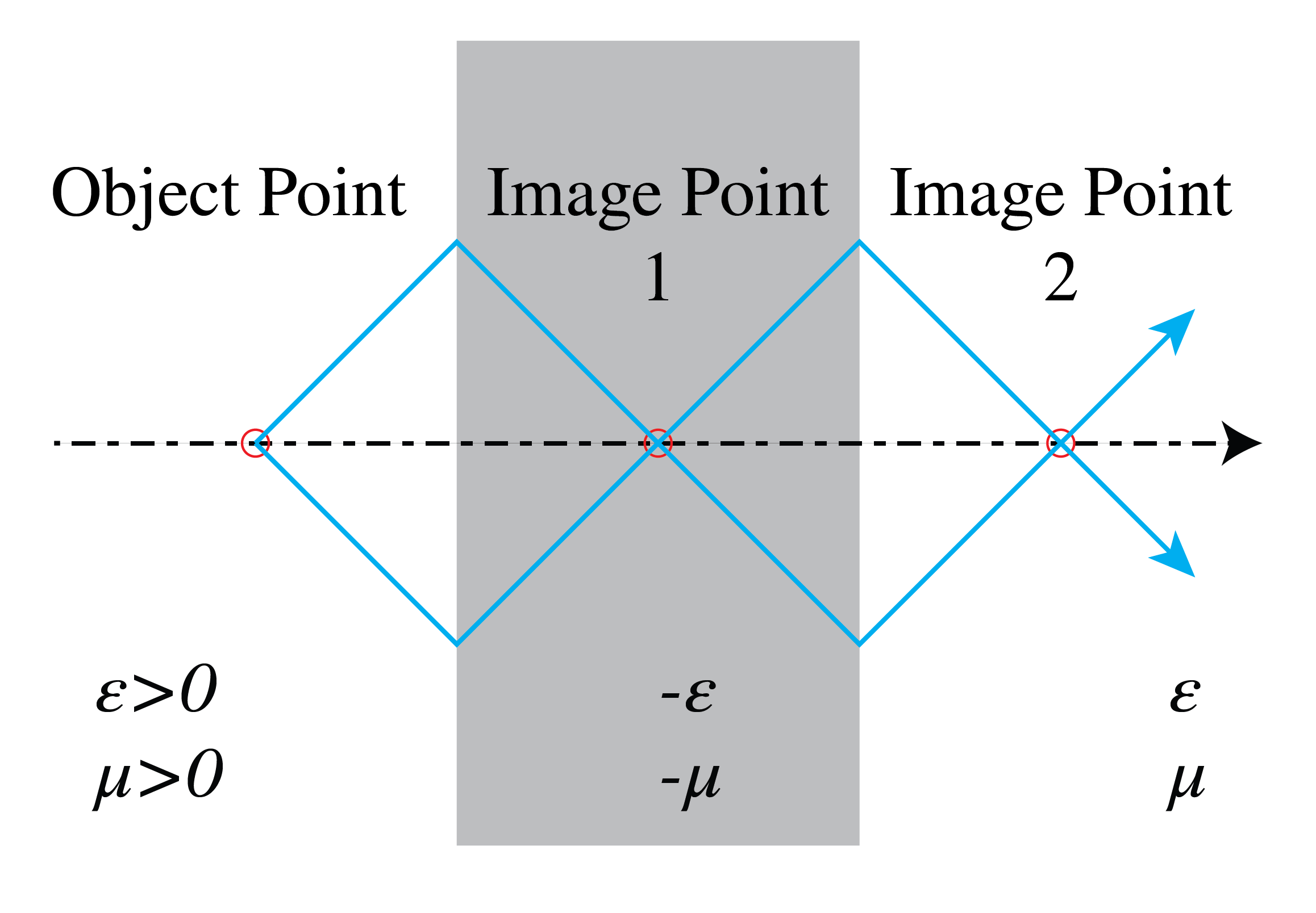
Figure 23:Pendry’s perfect lens consists of a slab of a material with negative permittivity and negative permeability such that their absolute values are equal to the positive permittivity and positive permeability of the surrounding medium. In the ideal lossless, exactly matched model, a source point has image points inside and beyond the slab.
The ideal slab proposal dates to 2000 [10]. Artificial composites can approximate a negative refractive index over a limited bandwidth, but finite loss and imperfect matching prevent a perfect image.
Hyperbolic materials. An anisotropic material can have permittivity components of opposite sign, giving a hyperbolic dispersion relation. In an ideal effective-medium model, some waves with transverse spatial frequency too high to propagate in ordinary media can propagate inside it. Real materials have absorption and a high-frequency cutoff set by their microscopic structure, so unlimited resolution and perfect imaging do not follow.
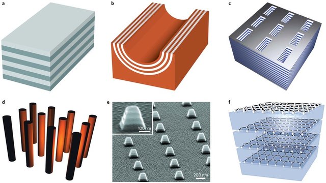
Figure 24:Examples of composite materials consisting of thin (sub-wavelength) layers of metals and dielectrics. These artificial materials are called metamaterials. (A. Poddubny, I. Iorsh, P. Belov, & Y. Kivshar, Hyperbolic Metamaterials, {N}at. {P}hoton., 7(12), 948-957 (2013)).
A few natural hyperbolic media exist for visible frequencies, but there are more in the mid-infrared. Researchers try to approximate hyperbolic media by metamaterials, made of, for example, multilayers consisting of alternating thin metallic and dielectric layers, so that the effective permittivity has the desired hyperbolic property. Also metallic nanopillars embedded in a dielectric are used.
Nonlinear effects. When the refractive index of a material depends on the local electric field, the material is nonlinear. At optical frequencies nonlinear effects are in general very small, but with a strong laser they can become significant. One effect is self-focusing, where the refractive index is proportional to the local light intensity. The locally higher intensity causes an increase of the refractive index, leading to a waveguiding effect due to which the beam focuses even more strongly. Hence the focused beam becomes more and more narrow while propagating, until finally the material breaks down.
Stimulated emission depletion microscopy (STED). Stefan Hell and Jan Wichmann proposed STED microscopy in 1994; later experiments demonstrated it, and Hell shared the 2014 Nobel Prize in Chemistry. An excitation spot raises fluorophores to an excited state. A doughnut-shaped depletion beam suppresses fluorescence around the central intensity zero by stimulated emission. Scanning the remaining small fluorescent region forms an image with resolution finer than the ordinary excitation spot. The attainable region depends on depletion intensity, fluorophore response, and noise; the doughnut’s dark center alone does not set the resolution. See the original proposal.
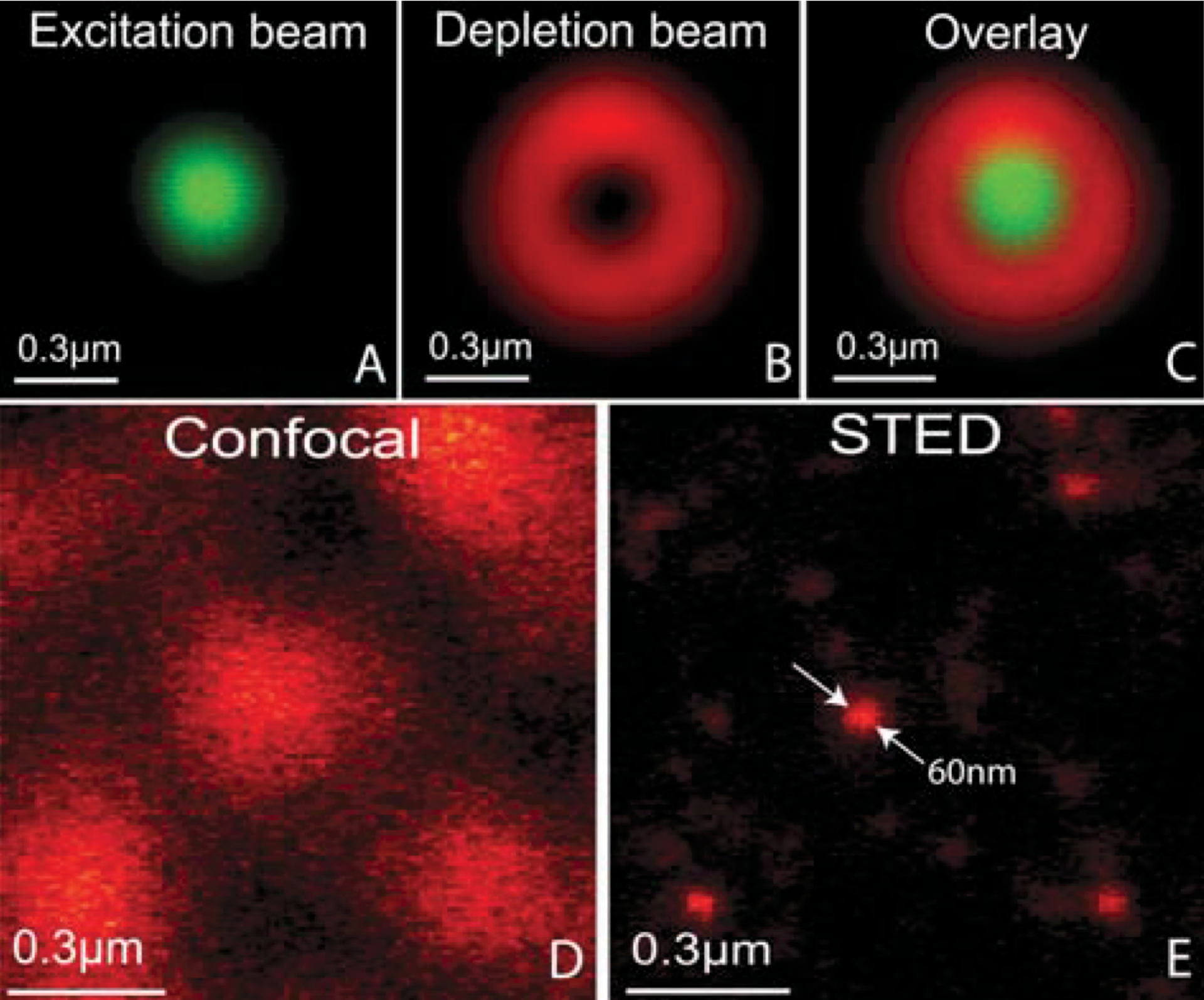
Figure 25:Spot used for excitation (top left) and for depletion (top middle). Fluorescence signal top right. In the lower figure the confocal image is compared to the STED image. (P.F. Rodriguez and al., Building a fast scanning stimulated emission depletion microscope, Materials Science (2012))
8Chapter Summary¶
Angular spectrum method decomposes fields into plane waves; propagation multiplies each by .
Rayleigh-Sommerfeld integral propagates fields by summing spherical wave contributions from each source point.
Fresnel approximation applies when the observation distance is much larger than the aperture size; quadratic phase approximation.
Fraunhofer approximation (far-field): The diffracted field is the Fourier transform of the aperture field.
Single slit: Intensity pattern ; first minimum at .
Circular aperture: Produces the Airy pattern; central disk radius .
Rayleigh criterion: Two point sources are resolved when the maximum of one coincides with the first minimum of the other.
Diffraction limit: A circular pupil has a first-zero Airy radius near ; finite numerical aperture and evanescent decay restrict conventional far-field imaging.
Lenses perform Fourier transforms: A lens in 2f-2f configuration gives the Fourier transform in its back focal plane.
Point-spread function (PSF): A point image; coherent object fields convolve with the amplitude PSF, while incoherent object intensities convolve with its squared modulus.
Super-resolution techniques (STED, near-field microscopy) can overcome the diffraction limit using special methods.
Sixty Symbols (2012) Basic explanation of Fourier transforms. Also see Section 3.
For a rigorous derivation see e.g. Goodman (2005), §3.3, §3.4, §3.5 - and Lecture Notes of Advanced Photonics, Delft University of Technology.
See the course Advanced Photonics given at TUDelft.
Sixty Symbols (2012) Basic explanation of the uncertainty principle (though in the context of quantum physics)
For a proof see Siegman (1986)
Goodman (2005), §5.2.2 - Several calculations on the Fourier transforming properties of lenses.
Hecht (2017) §10.2.6 ‘Resolution of imaging systems’.
Braat & Török (2019)
See Liu et al. (2008)
Pendry (2000)
- Poddubny, A., Iorsh, I., Belov, P., & Kivshar, Y. (2013). Hyperbolic metamaterials. Nature Photonics, 7(12), 948–957. 10.1038/nphoton.2013.243
- Sixty Symbols. (2012). Every picture is made of waves - Sixty Symbols. https://www.youtube.com/watch?v=mEN7DTdHbAU
- Sixty Symbols. (2012). Heisenberg’s Microscope - Sixty Symbols. https://www.youtube.com/watch?v=dgoA_jmGIcA
- Goodman, J. W. (2005). Introduction to Fourier Optics (3rd ed.). Roberts.
- Siegman, A. E. (1986). Lasers. University Science Books.
- Hecht, E. (2017). Optics (5th ed.). Pearson.
- Braat, J., & Török, P. (2019). Imaging Optics. Cambridge University Press.
- Liu, Z., Lee, H., Xiong, Y., Sun, C., & Zhang, X. (2008). Far-field optical hyperlens magnifying sub-diffraction-limited objects. Physical Review Letters, 100(12), 123904.
- Pendry, J. B. (2000). Negative refraction makes a perfect lens. Physical Review Letters, 85(18), 3966.