1Introduction
Although the model of geometrical optics helps us to design optical systems and explains many phenomena, there are properties of light that require a more elaborate model. For example, interference fringes observed in Young’s double-slit experiment or the Arago spot (Figure 3) indicate that light is more accurately modeled as a wave.
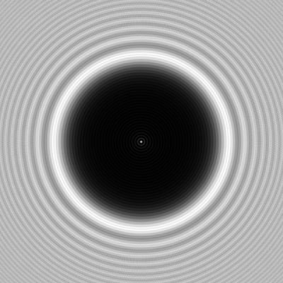
Arago spot observed with a 4 mm diameter circular disc. The bright central spot appears at the center of the disc’s shadow, demonstrating the wave nature of light through constructive interference of diffracted waves. Image captured at 1 m distance using 633 nm laser light.
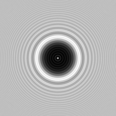
Arago spot observed with a 2 mm diameter circular disc. The relative size of the central bright spot increases compared to the disc diameter, as diffraction effects become more pronounced with smaller obstacles. Image captured at 1 m distance using 633 nm laser light.
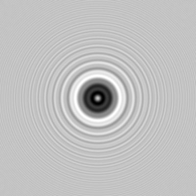
Figure 3:The Arago spot is the bright spot which occurs at the center of the shadow of a circular disc and which is caused by diffraction. The three images in this sequence show discs of diameter 4 mm, 2 mm, and 1 mm, respectively. The wavelength is 633 nm, and the intensity is recorded at 1 m behind the discs and has a width of 16 mm.
In this chapter we will study the wave model of light. It will be shown that the extent to which light can show interference depends on a property called coherence. For most of the discussion we will assume that all light has the same polarization, so that we can treat the fields as scalar. In the last section we will look at how polarization affects interference, as described by the Fresnel-Arago laws.
It is important to note that the concepts of interference and coherence are not just restricted to optics. Since quantum mechanics dictates that particles have a wave-like nature, interference and coherence also play a role in e.g. solid state physics and quantum information.
2Interference of Monochromatic Fields of the Same Frequency
Let us first recall the basic concepts of interference. What causes interference is the fact that light is a wave, which means that it not only has an amplitude but also a phase. Suppose for example we evaluate a time-harmonic field at two points
Here denotes the phase difference between the fields at the two points. If , or is a multiple of , the fields are in phase, and when they are added they interfere constructively
However, when , or more generally , for some integer , then the waves are out of phase, and when they are superimposed, they interfere destructively.
We can sum the two fields for arbitrary more conveniently using complex notation:
Adding gives
For and we retrieve the results obtained before. It is important to realize that what we see or detect physically (the ‘brightness’ of light) does not correspond to the quantities , . After all, and can attain negative values, while there is no such thing as ‘negative brightness’. What and describe are the fields, which may be positive or negative. The ‘brightness’ or the irradiance or intensity is given by taking an average over a long time of (as discussed in Chapter 1). We shall omit the factor . As explained in Chapter 1, we see and measure only the long time-average of , because at optical frequencies fluctuates very rapidly. We recall the definition of the time average over an interval of length at a specific time from Chapter 1:
where is a time interval that is the response time of a typical detector, i.e. which is extremely long compared to the period of visible light which is of the order of . For a time-harmonic function, the long-time average is equal to the average over one period of the field and hence it is independent of the time at which it is taken. Indeed for Eq. (5) we get
Using complex notation one can obtain this result more easily. Let
where
Then we find
hence
To see why this works, recall the time averaging formula and choose .
Remark. To shorten the formulae, we will omit in this chapter the factor in front of the time-averaged intensity.
Hence we define and , and we then find for the time-averaged intensity of the sum of and :
where and are the arguments of and and is the phase difference. The term is known as the interference term. In the famous double-slit experiment (which we will discuss in a later section), we can interpret the terms as follows: let us say is the field that comes from slit 1, and comes from slit 2. If only slit 1 is open, we measure intensity on the screen, and if only slit 2 is open, we measure . If both slits are open, we would not measure , but we would observe fringes due to the interference term .
The intensity Eq. (12) varies when the phase difference varies. These variations are called fringes. The fringe contrast is defined by
It is maximum and equal to 1 when the intensities of the interfering fields are the same. If these intensities are different the fringe contrast is less than 1.
More generally, the intensity of a sum of multiple time-harmonic fields all having the same frequency is given by the coherent sum
However, we will see in the next section that sometimes the fields are unable to interfere. In that case all the interference terms of the coherent sum vanish, and the intensity is given by the incoherent sum
3Coherence
In the discussion so far we have only considered monochromatic light, which means that the spectrum of the light consists of only one frequency. Although light from a laser often has a very narrow band of frequencies and therefore can be considered to be monochromatic, purely monochromatic light does not exist. One reason that light can not be perfectly monochromatic is that any source must have been switched on a finite time ago. Hence, all light consists of multiple frequencies and therefore is polychromatic. Classical light sources such as incandescent lamps and also LEDs have relatively broad frequency bands. The question then arises how polychromatic light behaves differently from idealized monochromatic light. To answer this question, we must study the topic of coherence. One distinguishes between two extremes: fully coherent and fully incoherent light, while the degree of coherence of practical light is somewhere in between. A broader frequency band generally gives a shorter temporal coherence time. Spatial coherence also depends on source size and geometry. It is a very important observation that no light is actually completely coherent or completely incoherent. All light is partially coherent, but some light is more coherent than others.
An intuitive way to think about these concepts is in terms of the ability to form interference fringes. For example, with laser light, which usually is almost monochromatic and hence coherent, one can form an interference pattern with clear maxima and minima in intensities using a double slit, while with sunlight (which is incoherent) this is much more difficult. Every frequency in the spectrum of sunlight gives its own interference pattern with its own frequency dependent fringe pattern. These fringe patterns wash out due to superposition and the total intensity therefore shows little fringe contrast, i.e. the coherence is less. However, it is not impossible to create interference fringes with natural lightYoung, 1804. The trick is to let the two slits be so close together (of the order of ) that the difference in distances from the slits to the sun is small enough for the fields in the slits to be sufficiently coherent to interfere. For one point source, a path difference determines the time delay between fields at two observation points. For an extended source, distance matters as well: it changes the angular size of the source and thus the spatial coherence.
3.1Coherence of Light Sources
In a conventional light source such as a gas discharge lamp, photons are generated by spontaneous emission with energy equal to the energy difference between certain electronic states of the atoms of the gas. These transitions have a duration of the order of 10-8 to . Because the emitted wave trains are finite, the emitted light does not have a single frequency; instead, there is a band of frequencies around a center frequency with width roughly equal to the reciprocal of the duration of the wave train. This spread of frequencies is called the natural linewidth. Random thermal motions of the molecules cause further broadening due to the Doppler effect. In addition, the atoms undergo collisions that interrupt the wave trains and therefore further broaden the frequency spectrum.
We first consider a single emitting atom. When collisions are the dominant broadening effect and these collisions are sufficiently brief, so that any radiation emitted during the collision can be ignored, an accurate model for the emitted wave is a steady monochromatic wave train at frequency at the center of the frequency band, interrupted by random phase jumps each time that a collision occurs. The discontinuities in the phase due to the collisions cause a spread of frequencies around the center frequency. An example is shown in Figure 4. The average time between the collisions is typically less than 10-10 s which implies that on average between two collisions roughly 105 harmonic oscillations occur and that during an atomic transition of the order of a hundred collisions may occur. A coherence time characterizes the delay over which a field remains strongly correlated with itself; its precise value depends on the chosen correlation threshold. In this collision-dominated model it is of the order of the mean time between collisions, , which may be about 10-10 s.
To understand coherence and incoherence, it is helpful to use this model for the emission by a single atom as harmonic wave trains of many thousands of periods interrupted by roughly a hundred random phase jumps. Due to the random phase jumps, the interference term of the sum of harmonic wave trains emitted by two atoms, when integrated over the relatively long integration time of a detector, becomes a sum over integrals over time intervals of average length :
where the sum is over roughly one hundred random phase jumps during the total duration of the wave trains. The random phase jumps lead to cancellation of the integrals and hence the interference term vanishes. We conclude that over the integration time of typical detectors
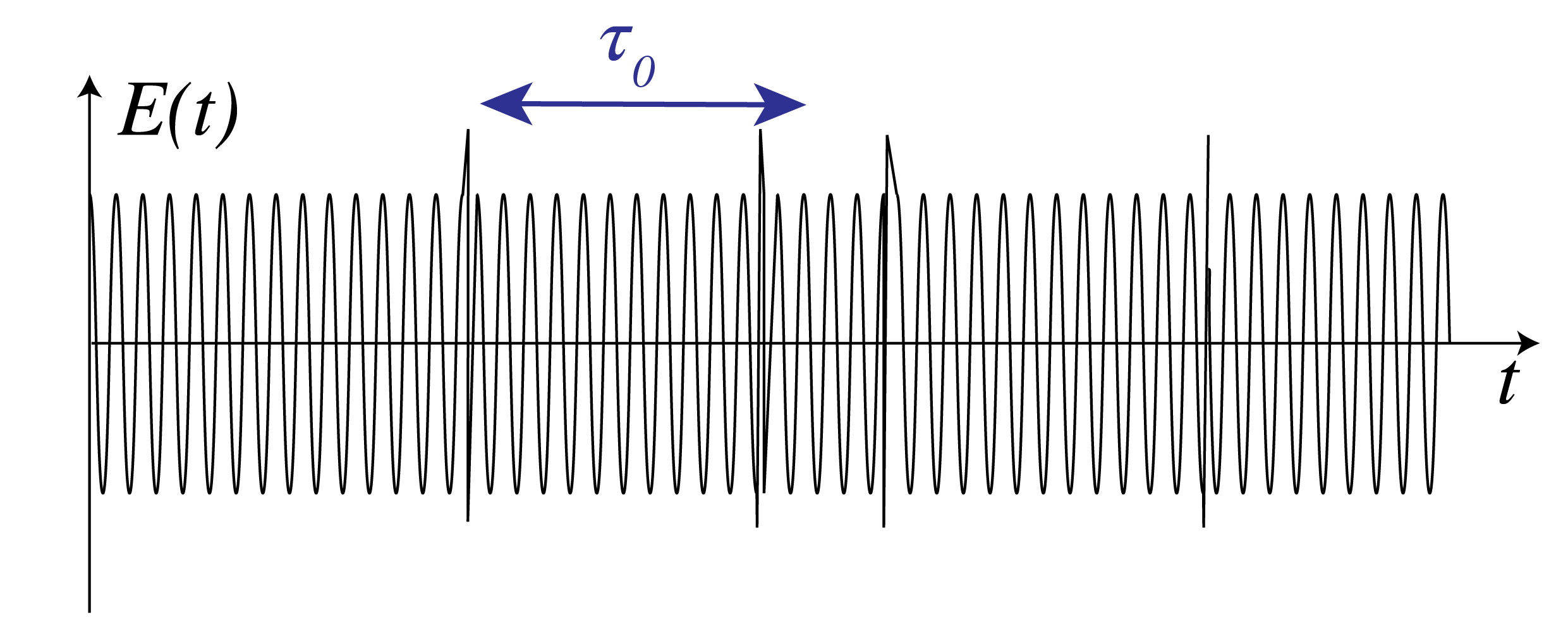
Figure 4:The electric field amplitude of the harmonic wave train radiated by a single atom at the center frequency . The vertical lines are collisions separated by periods of free flight with mean duration . The quantity , which is the number of periods in a typical wave train, is chosen unrealistically small (namely 60, whereas a realistic value would be 105) to show the random phase changes.
For a narrow, smooth spectral line, the coherence time is of order the reciprocal bandwidth. If linewidth is quoted as an ordinary frequency width , an estimate is
The corresponding coherence length is estimated by
For a narrow band in vacuum, gives, to first order in bandwidth,
where and are the wavelength and the frequency at the center of the line. Hence,
Order-of-magnitude coherence lengths and times of several sources are listed in Table 1. For a laser, the linewidth is extremely small and the coherence time very long. This is because the photons in a laser are not generated predominantly by spontaneous emission as they are in classical sources, but instead by stimulated emission. Lasers are discussed in Lasers.
Table 1:Coherence time and coherence length of several sources
| Source | Mean wavelength | Linewidth | Coherence Length | Coherence Time |
|---|---|---|---|---|
| Mid-IR (3-5 ) | 4.0 | 8.0 | s. | |
| White light | 550 nm | nm | nm | s. |
| Mercury arc | 546.1 nm | nm | mm | s. |
| discharge lamp | 605.6 nm | nm | 0.3 m | s. |
| Stabilized He-Ne laser | 632.8 nm | nm | 400 m | s. |
3.2Polychromatic Light
When dealing with coherence one has to consider fields that consist of a range of different frequencies. Let be the real-valued field component. It is always possible to write as an integral over time-harmonic components:
where is the complex amplitude of the time-harmonic field with frequency . When there is only a certain frequency band that contributes, then for outside this band. We define the complex time-dependent field by
Then
Remark: The complex field now contains the time dependence in contrast to the notation used for a time-harmonic (i.e. single frequency) field introduced in Chapter 2, where the time-dependent was a separate factor.
We now compute the intensity of polychromatic light. The instantaneous energy flux is (as for monochromatic light) proportional to the square of the instantaneous real field: . We average the instantaneous intensity over the integration time of common detectors. As stated before, this integration time is very long compared to the period at the center frequency of the field. Using Eq. (6) and
we get
where the averages of and are zero because they are fast-oscillating and go through many cycles during the integration time of the detector. In contrast, has a DC-component which does not average to zero.
Remark: In contrast to the time-harmonic case, the long time average of polychromatic light depends on the time at which the average is taken. However, we assume in this chapter that the fields are emitted by sources that are stationary. The property of stationarity implies that the average over the time interval of long length does not depend on the time at which the average is taken. Many light sources, in particular conventional lasers, are stationary. (However, a laser source which emits short high-power pulses cannot be considered as a stationary source). We furthermore assume that the fields are ergodic, which means that taking the time-average over a long time interval amounts to the same as taking the average over the ensemble of possible fields. It can be shown that this property implies that the limit in Eq. (6) indeed existsMandel & Wolf, 1995.
We use for the intensity again the expression without the factor in front, i.e.
The time-averaged intensity has hereby been expressed in terms of the time-average of the squared modulus of the complex field.
Quasi-monochromatic field. If the width of the frequency band is very narrow compared to the center frequency , we speak of a quasi-monochromatic field. In the propagation of quasi-monochromatic fields, we use the formula for time-harmonic fields at . The quasi-monochromatic assumption simplifies the computations considerably and will therefore be used frequently.
4Temporal Coherence and the Michelson Interferometer
To investigate the time coherence of a field at a certain point , we let the field at that point interfere with a delayed copy of itself, i.e. we let interfere with . Because, when studying temporal coherence, the point is always the same, we omit it from the formula. Furthermore, for easier understanding of the phenomena, we assume for the time being that the field considered is emitted by a single atom (i.e. a point source).
Temporal coherence is closely related to the spectral content of the light: if the light consists of fewer frequencies (think of monochromatic light), then it is more temporally coherent. To study the interference of with , a Michelson interferometer, shown in Figure 5, is a suitable setup. The light that goes through one arm takes time to reach the detector, while the light that goes through the other (longer) arm takes time , which means that it was radiated earlier. Therefore, the detector observes the time-averaged intensity . As remarked before, this averaged intensity does not depend on the time the average is taken; it only depends on the time difference between the two beams.
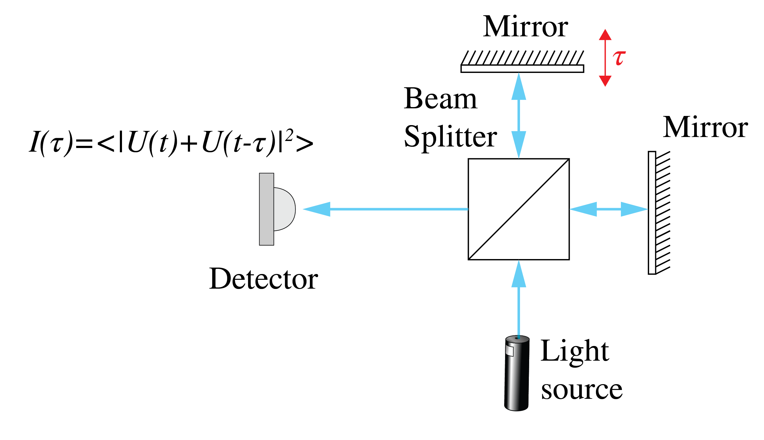
Figure 5:A Michelson interferometer to study the temporal coherence of a field. A beam is split in two by a beam splitter, and the two beams propagate over different distances, corresponding to a time difference , and then interfere at the detector.
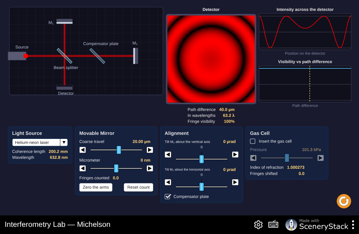
Figure 6:A physical-optics Michelson: move a mirror, change the source coherence length, and watch fringe visibility collapse. The intensity versus delay is the self-coherence function of this section, measured rather than postulated.
Interactive simulation: Interferometry Lab
We have
The detected intensity varies with the difference in arm length.
So far we have considered a field that originates from a single atom. The total field emitted by an extended source is the sum of fields corresponding to all atoms . As has been explained already, fields from independent atoms have cross terms that vanish after averaging. But the field emitted by an atom can interfere with the delayed field of that same atom and for every atom the interference is given by the same expression Eq. (27). If the atoms contribute equally and share the same spectral shape, the total intensity is the single-atom result multiplied by their number. More generally, their intensities add, each with its own self-coherence term.
The self coherence function is defined by
The intensity of is
The complex degree of self-coherence is defined by:
Using the Cauchy–Schwarz inequality it can be shown that this is a complex number with modulus between 0 and 1:
The observed intensity can then be written:
We consider two special cases.
Suppose is a monochromatic wave
In that case we get for the self-coherence
and
Hence the interference pattern is given by
So for monochromatic light we expect to detect a cosine interference pattern, which shifts as we change the arm length of the interferometer (i.e. change ). No matter how large the time delay , a clear interference pattern should be observed.
Next we consider what happens when the light is a superposition of two frequencies:
where , and is the integration time of the detector. Then:
where in the second line the time average of terms that oscillate with time is set to zero because the averaging is done over a time interval satisfying . Hence, the complex degree of self-coherence is:
and Eq. (32) becomes
The interference term is the product of the function , which is a rapidly oscillating function of , and a slowly varying envelope . The visibility envelope vanishes at some delays and then revives periodically. Thus this ideal two-line source has no single coherence decay time. Increasing line separation brings the first zero closer to zero delay[3][4]. For a smooth, broad spectrum the correlation envelope commonly narrows as bandwidth increases. A practical coherence time needs a stated visibility threshold or linewidth convention. We conclude with some further interpretations of the degree of self-coherence .
Remarks.
In stochastic signal analysis is called the autocorrelation of . Informally, one can interpret the autocorrelation function as the ability to predict the field at time given the field at time .
For a stationary field, the Wiener–Khinchin theorem relates the self-coherence function to the power spectral density. With the Fourier convention used here,
The Fourier relation shows that the larger the spread of the frequencies of (i.e. the larger the bandwidth), the more sharply peaked is. Thus, the light gets temporally less coherent when it consists of a broader range of frequencies. Measuring the spectral power density with a spectroscope and applying an inverse Fourier transform is an alternative method to obtain the complex self-coherence function.
5Spatial Coherence and Young’s Experiment
Temporal coherence concerns the coherence of the field in one point. The absolute value of the degree of self coherence Eq. (30) quantifies how strong the interference is of the field in the point of interest with the field in that same point at a later time. In contrast, spatial coherence is concerned with determining how coherent the fields in two different points are. This is done by letting the fields interfere using a mask with two small holes at the positions of the points of interest and observing the fringe contrast at a distant screen (Young’s experiment).
While for temporal coherence we used a Michelson interferometer, the natural choice to characterize spatial coherence is Young’s experiment, because it allows the fields in two points , which are separated in space to interfere with each other.
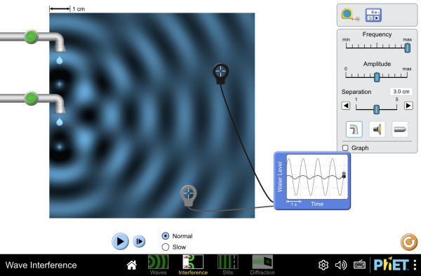
Figure 7:Young’s geometry with slit separation, slit width, and wavelength under direct control. Switch between one slit and two: the fringe contrast on the screen is the spatial-coherence diagnostic used throughout this section.
Interactive simulation: Wave Interference
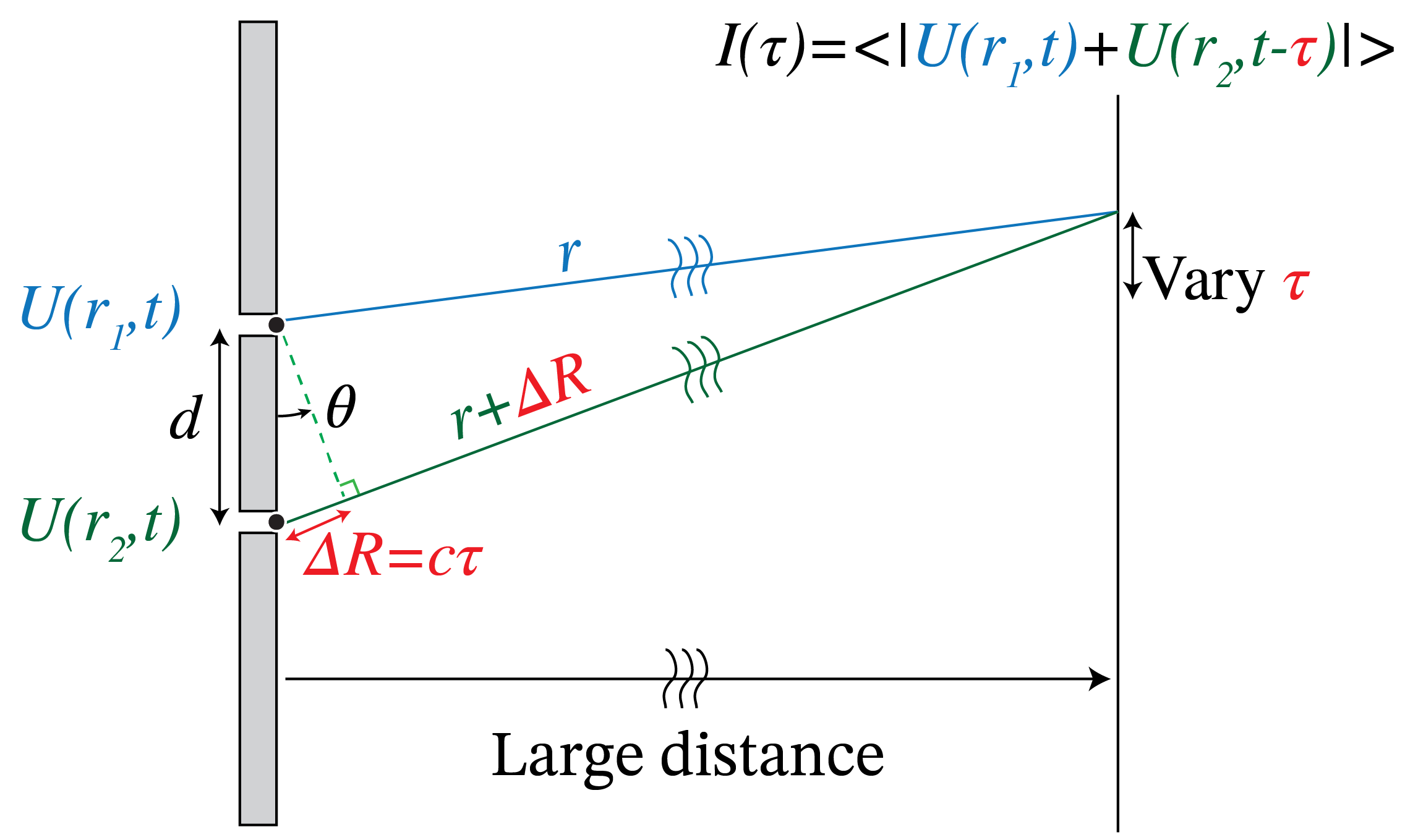
Figure 8:The spatial coherence of light from an extended source.
Let and be the position vectors of the points and , respectively. We write the complex field in as a superposition of monochromatic fields as in Eq. (22):
The reason for doing this is that for a monochromatic field in the pinhole, i.e. a field with a well defined frequency, we can derive the disturbance in any point behind the mask. In fact, according to the Huygens-Fresnel Principle, a monochromatic disturbance with frequency in the pinhole at generates a radiating spherical wave with the same frequency . Apart from a common diffraction and obliquity factor, its field at is proportional to
Here is a common complex coupling factor that includes pinhole area, diffraction normalization, and the obliquity factor. We treat it as frequency independent over a narrow band and approximately equal for the two identical pinholes in the far field. The frequency remains in the propagation phase because even a small frequency change can produce a substantial phase change over a long path. The total field in due to the pinhole at is obtained by integrating the monochromatic components over frequency:
In words:
For the field in due to pinhole 2 we have similarly
The total field in is the sum . Because of the difference in propagation distance , there is a time difference between the times when the two fields were emitted by the two pinholes so that they arrive at a given time at point on the screen in Figure 8. This time difference is given by
Furthermore, the amplitudes are reduced by a factor proportional to the reciprocal distance which is different for the two fields. But if the distance of the screen to the mask is large enough, we may assume these factors to be the same and then omit them. Using Eq. (46), the interference pattern on the screen is then, apart from a constant factor, given by
The second line uses stationarity: delaying a field does not change its mean intensity. We define the mutual coherence function by:
With the intensities
the complex degree of mutual coherence is defined by
It can be proved using Bessel’s inequality that
We can now write Eq. (47) as
By varying the point over the screen we can vary and by measuring the intensities we can determine the real part of and hence the fringe contrast observed on the screen.
As an example, consider what happens when is a monochromatic field
In that case
and
So we get
where . In this case has modulus 1, as expected for a monochromatic field. The intensity on the screen becomes
The fields are fully coherent because . Their fringe contrast is , reaching 1 only when the pinhole intensities are equal. If , then interference maxima occur for
Because , and , we find that maxima occur when
For a large distance between the screen and the mask (in the Fraunhofer limit), these path length differences correspond to directions of the maxima given by the angles (see Figure 8):
where is the distance between the slits and is an integer[5].
Remarks.
The mutual coherence is the cross-correlation of the two signals and .
As remarked above, by moving the point of observation over the screen, one can obtain the real part of the complex degree of mutual coherence. To derive also the imaginary part, one can put a piece of glass behind one of the pinholes with thickness such that for the center frequency an additional phase difference of is obtained between the fields in and . If the frequency band is sufficiently narrow this phase difference applies to a good approximation to all frequencies in the band.
6More on Spatial Coherence
We first consider the case that the source is so small (e.g. a single emitting atom) that it can be considered to be a point source . The correlation of the fields at two points and then depends on the travel-time difference from . A path difference much smaller than the source coherence length generally gives high visibility; a much larger difference gives low visibility for a smooth broad spectrum.
An extended classical light source consists of a large set of emitting point sources that emit by spontaneous emission. As we have explained in Section 3.1, the wave trains emitted by different atoms (point sources) in the source suffer random phase jumps due to e.g. collisions and therefore their averaged cross terms vanish. Such a light source is called spatially incoherent. For a spatially incoherent light source, the spatial coherence in any two points and is determined by measuring the fringe contrast on a distant screen when a mask is used that is perpendicular to the mean direction of propagation of the light and which contains pinholes at and . The fringe contrast and hence the mutual coherence at and are determined by two effects:
First of all it is determined by how coherent the contributions of the individual point sources in the extended source to the total fields at and are. This coherence is determined by the extent to which the difference between the distance of to and of to is smaller than the coherence length. If these differences in distances are for all point sources larger than the coherence length, the fringe contrast on the screen in Young’s experiment will be very low and hence the mutual coherence is very low.
The second effect is the size of the extended source. Even if for all point sources in the source the fields in and are coherent, the coherence of the total fields at and due to the entire source can be small. As we know, the cross terms between independent source points vanish after averaging. Hence the intensity observed in Young’s experiment is the sum of the intensities due to the individual point sources in the extended source. The total coherence can still be low because the fringe patterns from different source points shift relative to one another and cancel on averaging. The shift of the fringe patterns is due to the different positions of the point sources in the extended source, which cause the phase difference between the fields in and to vary with the point sources.
For a distant source, a small product of angular source size and pinhole separation keeps path delays small. This alone does not prevent fringes from different source points from canceling when their intensities are added.
To show this we consider two mutually incoherent point sources and in the plane. Their mutual coherence function satisfies:
where is the self-coherence which we assume to be the same for both point sources. has a characteristic width set by the source spectrum. For a smooth broad spectrum its envelope generally decreases with delay, although it need not be monotonic. Eq. (61) expresses the fact that two point sources are mutually incoherent. Using the fact, based on the assumption that the source is stationary, that the long-time average does not depend on the origin of time, we find:
Furthermore, for : , which is the intensity of either source.
We assume for convenience that the two points , are at a large distance from the two point sources and that the line is parallel to the line joining the two point sources as shown in Figure 9. We will compute the mutual coherence for zero time delay (we can also compute the mutual coherence for more general time delays , i.e. , but it will suffice for our purpose to take ). The fields in and are the sum of the fields emitted by and . Since and are point sources they emit spherical waves. Therefore, similarly to Eq. (44) we find that the field in is proportional to
and
where we omitted the constant factors in front of Eq. (44).
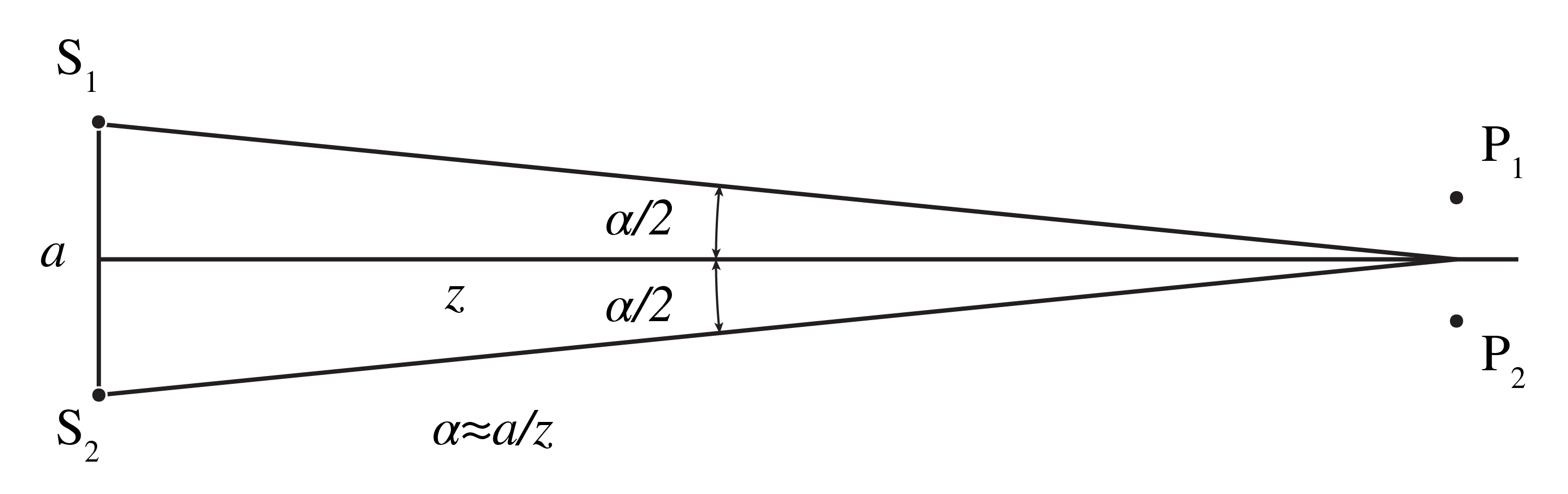
Figure 9:Two incoherent point sources , at a distance from each other and two points , in a plane at large distance from the point sources.
For sufficiently large , all distances in the denominators may be replaced by . We absorb their common amplitude factor, including the coupling coefficient, into the field normalization. By substituting Eq. (64) and Eq. (65) into Eq. (48) with , we find for the mutual coherence of and :
Now we use Eq. (61) and Eq. (62) to get
Similarly,
Because the width of the self-coherence function is set by the coherence time , result Eq. (67) confirms that for the fields in and to be coherent, the path difference from each source point to and should be small compared with the coherence length for that source contribution to retain appreciable visibility. To express the result in terms of the angle subtended by the source at the midpoint of we choose coordinates such that for . If the distance to the source is so large that and are almost parallel, we see from Figure 9 that
Similarly,
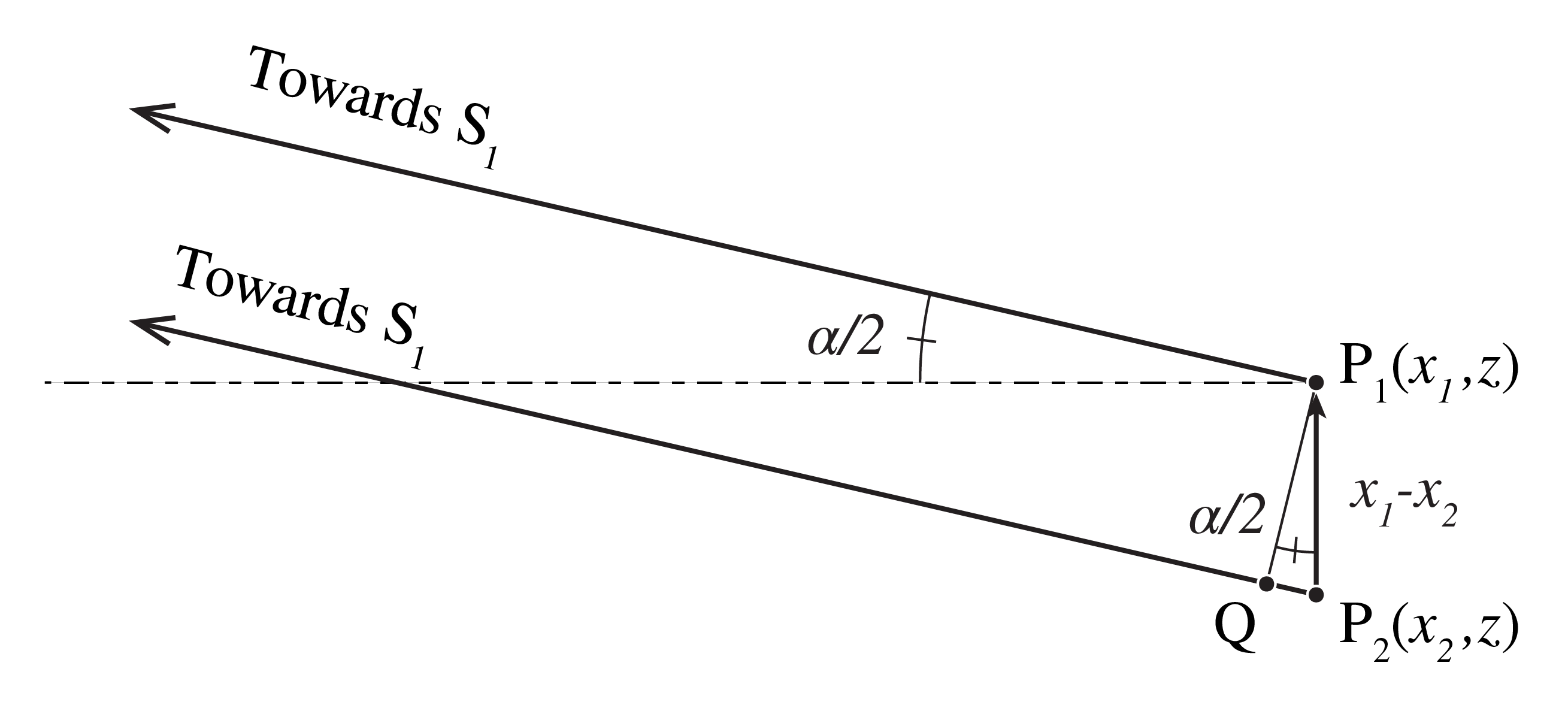
Figure 10:For very large, and are almost parallel and .
Hence, with , Eq. (67) becomes
The argument of shows how finite bandwidth reduces each source contribution as its path difference grows. The sum of those contributions can also cancel because their phases differ, even when each is individually coherent.
At fixed pinhole separation, moving a source farther away reduces its angular size. Near zero angular size the contributions have nearly the same phase and spatial coherence approaches one. For a discrete source, visibility can have additional zeros and revivals at larger angular sizes.
As an example, consider quasi-monochromatic light for which (see Eq. (34)):
Here is the center frequency. This idealization treats each source as monochromatic over the delays of interest, so its temporal coherence length is effectively much larger than all relevant path differences. Hence the only remaining criterion for coherence of the total fields in and is that the fringe patterns due to the different point sources in Young’s experiment sufficiently overlap. Indeed, in this case of very long coherence time we have
and hence the degree of mutual coherence is:
For these two equal point sources, with baseline , the first visibility zero occurs at . This is a first null, not a maximum allowed separation: revives at larger baselines. A continuous source has a different visibility function.
6.1Example: Solar coherence across a baseline
The Sun has an angular diameter of about radians, or . The two-point-source cosine derived above does not describe a filled solar disk. For a uniformly bright circular disk observed through a narrow spectral band, the van Cittert–Zernike result gives the modulus of the spatial degree of coherence at baseline :
where is a Bessel function. The first zero occurs at . At , this is about . A baseline of still gives appreciable visibility; it is not a hard maximum coherence distance. Solar limb darkening and finite bandwidth alter the precise visibility curve.
7Stellar Interferometry
The dependence of spatial coherence on source angular size is used in stellar interferometry. It works as follows: we want to know the size of a certain star. The size of the star, being an extended spatially incoherent source, determines the spatial coherence of the light we receive on earth. Thus, by measuring the interference of the light collected by two transversely separated telescopes, one can effectively create a double-slit experiment, with which the degree of spatial coherence of the starlight on Earth can be measured, and thereby the angle which the star subtends on earth. A longer telescope baseline probes finer angular structure (see Eq. (74)). If the distance of the star is measured independently, for example by parallax, its physical size follows from its angular size.
With measurements of complex visibility, including phase, across enough telescope baselines, one can reconstruct the projected brightness distribution of the star. The van Cittert–Zernike theorem relates that visibility to the Fourier transform of angular source brightness. Measuring fringe contrast alone gives only the modulus of visibility and does not by itself determine a unique image.
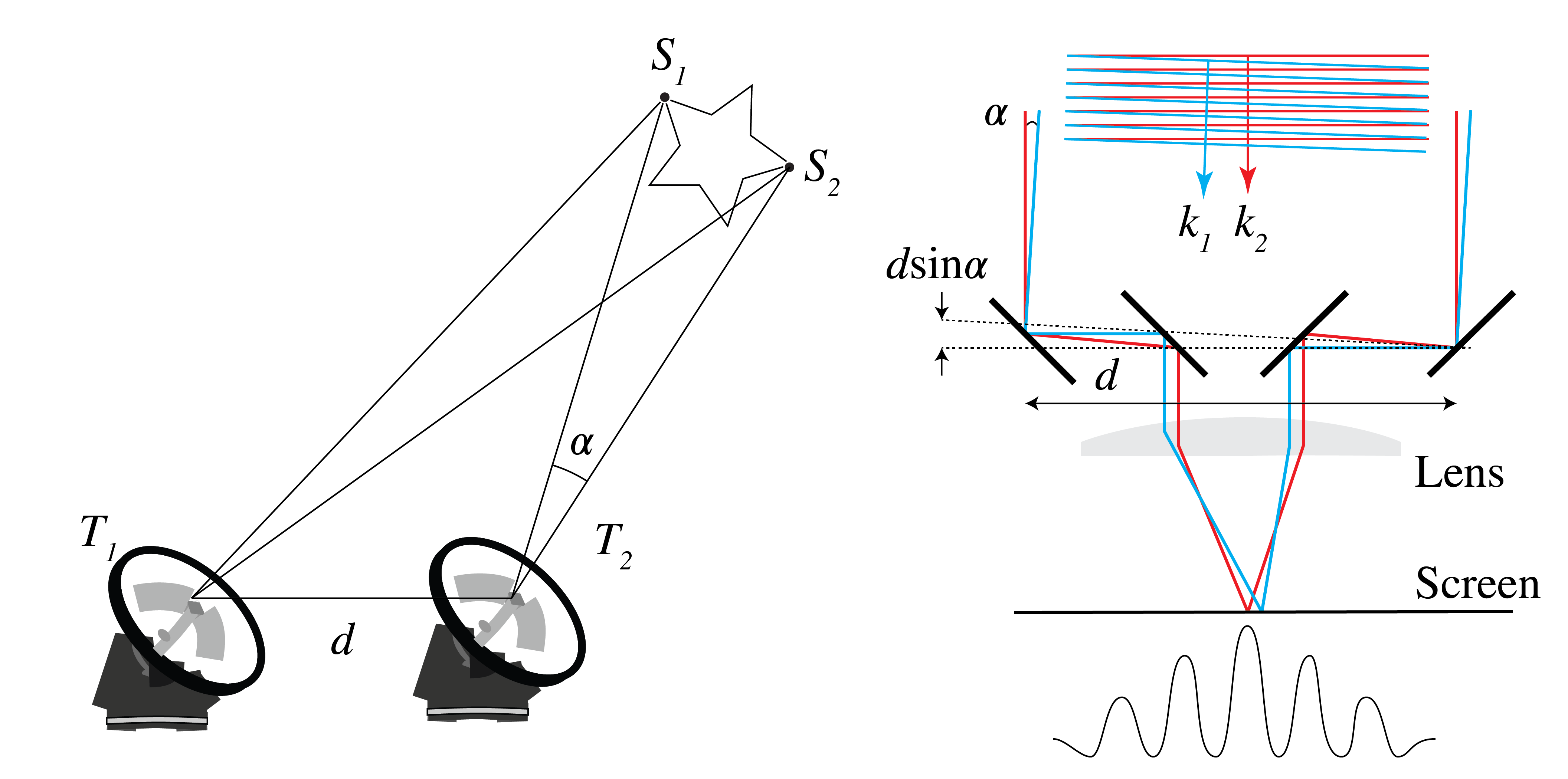
Figure 11:Left: a stellar interferometer with two telescopes that can be moved around to measure the interference at many relative positions. Right: single telescope with two outer movable mirrors. The telescope can move around its axis. The larger the distance the higher the resolution.
8Fringe contrast
We have seen that when the interference term vanishes, no fringes form, while when this term is nonzero, there are fringes. The fringe contrast is expressed directly in measurable intensities. Given some interference intensity pattern as in Figure 12, the fringe contrast is defined as
For example, if we have two perfectly coherent, monochromatic point sources emitting the fields , with intensities , , then the interference pattern is given by Eq. (57):
We then get
so
In case , we find .
In contrast, when and are completely incoherent, we find
from which follows
which gives .
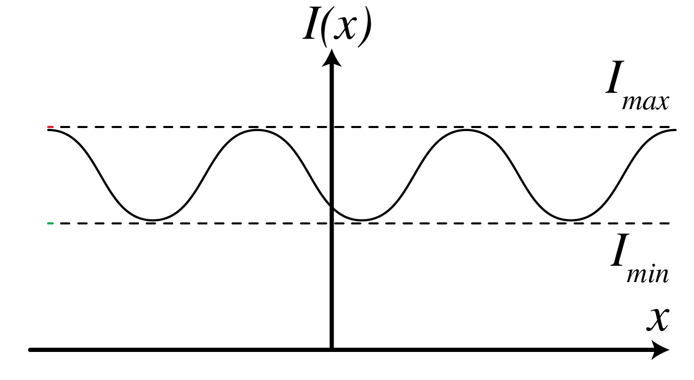
Figure 12:Illustration of and of an interference pattern that determines the fringe contrast .
9Fabry–Perot resonator
Figure 13:A Fabry–Pérot cavity with adjustable mirror reflectance, spacing, and absorption. Watch finesse, free spectral range, and resolving power update as the transmission peaks sharpen.
Interactive simulation: Interferometry Lab
An interferometer combines fields whose phase difference contains information about an optical path. Young’s slits and Lloyd’s mirror divide a wavefront; a Michelson interferometer divides amplitude. A Fabry–Perot etalon divides amplitude repeatedly between two parallel reflecting surfaces. It is used as a high-resolution spectrometer and as an optical cavity.
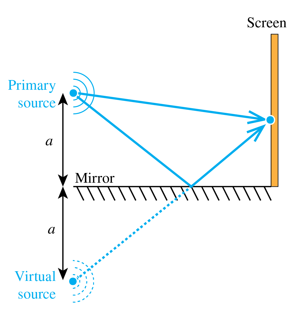
Figure 14:Lloyd’s mirror is an example of wavefront division.
The figure below shows a slab of thickness and refractive index , between media and . Snell’s law determines the internal angle . In the derivation below, specialize to a lossless, symmetric etalon: the outside media are identical, the two mirrors have the same power reflectance , their reflection phases are neglected or absorbed into the cavity phase, and polarization and angle are held fixed. These assumptions make incident and transmitted powers directly comparable. Absorption or unequal mirrors require different peak heights and a modified transmission formula.
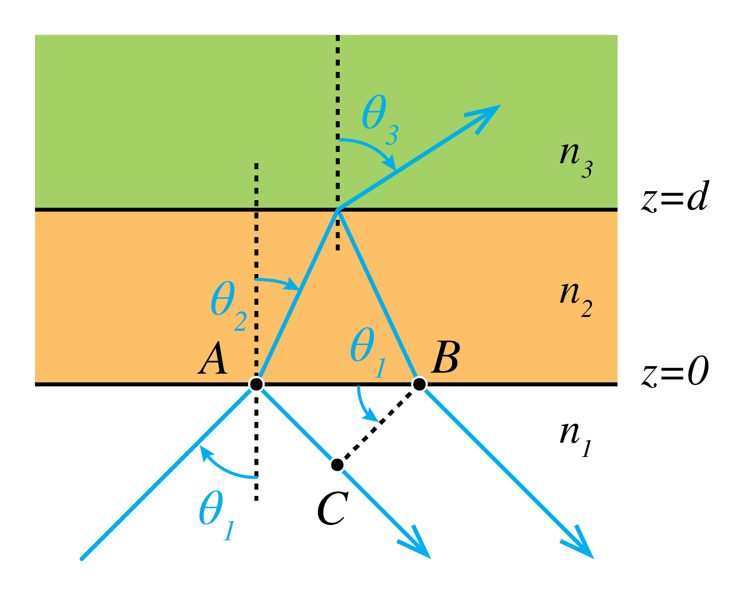
Figure 15:Three-layer geometry of the Fabry–Perot etalon. The formulas below use identical outside media and mirror reflectances.
Let , where is the vacuum wavelength. The phase gained across the slab in the normal direction is
Successive transmitted beams have a round-trip phase difference . With the electric-field phase convention , the round-trip amplitude factor is . For a symmetric lossless etalon, the transmitted amplitude, normalized to unit incident amplitude, is
The numerator combines the two mirror transmissions. Their possible common phase has no effect on transmitted power. Taking the squared modulus gives the Airy transmission law
Here is the coefficient of finesse, distinct from the finesse defined below. Energy conservation gives the reflected power fraction
Thus . At resonance, transmission is unity and reflection vanishes in this ideal symmetric model. Real absorption and mirror asymmetry reduce the transmission peak.
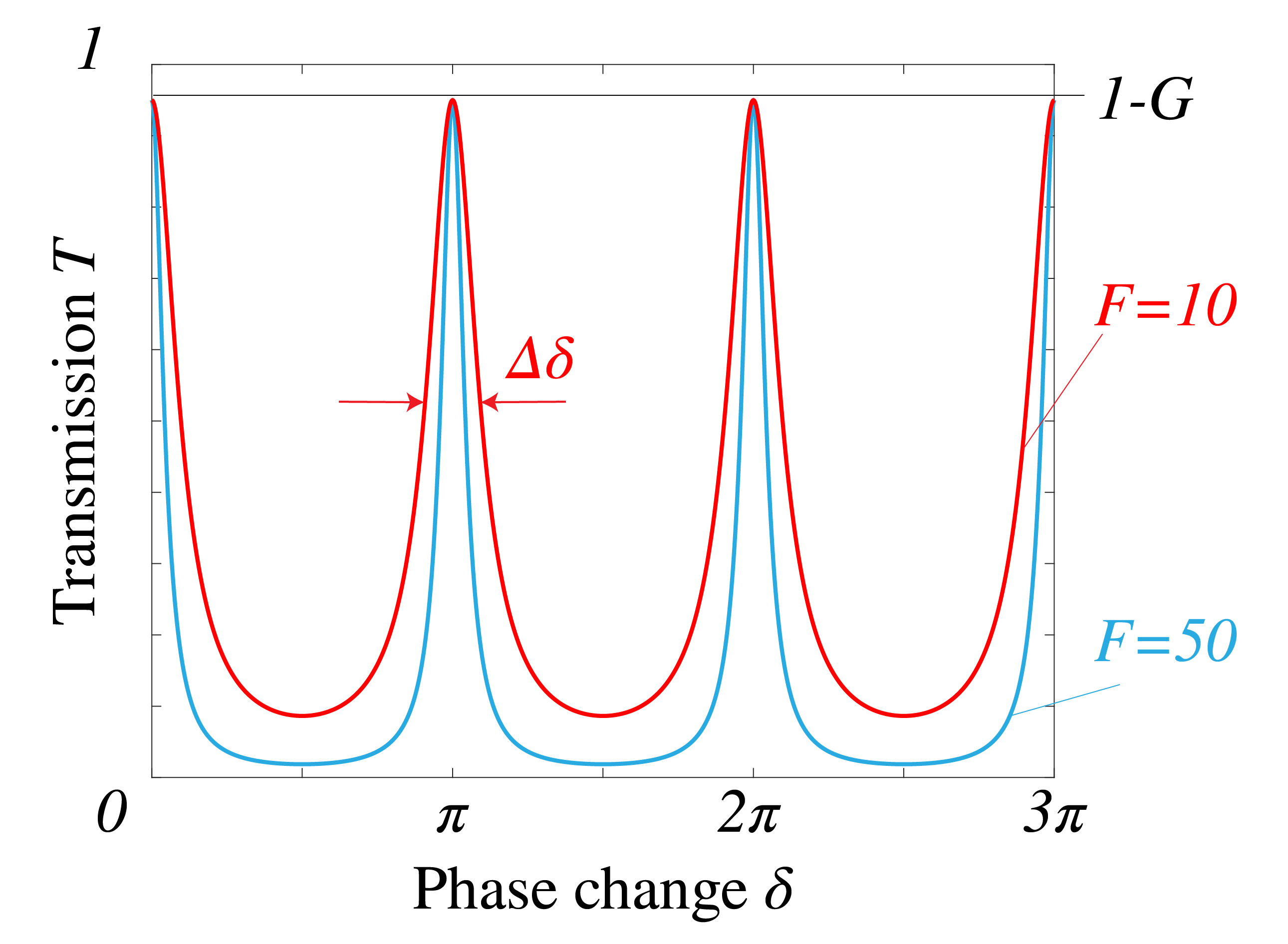
Figure 16:Transmission versus single-pass phase for two values of . The plotted symmetric case has peak transmission 1.
Resonance occurs when the round-trip phase is a multiple of :
Equivalently, when dispersion can be neglected over one peak,
The free spectral range is the separation between neighboring orders:
The frequency expression assumes negligible material and mirror-phase dispersion over the interval. With dispersion, obtain the spacing from the frequency derivative of the full round-trip phase.
For , the full width at half maximum of one isolated peak is
The finesse is the ratio of free spectral range to this width:
Near order , the fractional wavelength width is approximately . The wavelength resolving power is therefore
Also , so the ratio of free spectral range to linewidth is . Raising improves local resolving power but narrows the unambiguous wavelength interval.
9.1Example: Fabry–Perot resolution
For normal incidence, and give . If each mirror has , then and . The resolving power is approximately , assuming negligible absorption and dispersion. This example uses the high-finesse approximation.
10Interference and polarization
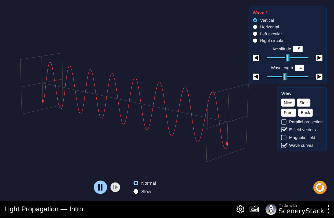
Figure 17:Rotate a polarizer and compare the transmitted intensity of two field components. Their ability to form fringes depends on both polarization overlap and phase correlation.
Interactive simulation: Light Propagation
Light is a vector field. For a detector that does not analyze polarization, the intensity of two superposed complex fields is proportional to
The averaging includes the detector response. The dot product describes polarization overlap; the correlation describes whether the relative phase persists during averaging. Both are needed for visible interference.
First Fresnel–Arago principle. Orthogonally polarized fields have zero dot product, so they produce no interference term at a polarization-insensitive detector. A subsequent polarizer can project both fields onto the same direction, after which interference is possible if the projected fields remain correlated.
Second Fresnel–Arago principle. Parallel polarized components can interfere if they are mutually coherent. Two copies made from the same natural-light field can show fringes when the path delay is within its coherence time. Two independent natural-light sources generally have no stable interference term even if their polarizations are made parallel.
Third Fresnel–Arago principle. The two orthogonal components of ideal unpolarized natural light are mutually uncorrelated. Splitting them and rotating one into alignment does not create the missing correlation, so no stable fringes appear. The conclusion assumes the original light is unpolarized; a polarized source can have correlated components.
These principles explain why a shared polarization was useful in the scalar calculations above, while also showing that shared polarization alone cannot guarantee fringe visibility.
11Chapter Summary
Interference occurs when two or more coherent waves overlap; the resulting intensity depends on their relative phase.
Temporal coherence measures how well a wave correlates with itself over time; it is related to bandwidth by .
Coherence length is the path difference over which fringes remain visible.
Spatial coherence measures correlation between different points in a wave field at the same time.
Young’s double-slit experiment: Fringe spacing , where is screen distance and is slit separation.
Michelson interferometer measures path differences and coherence length and is used for spectroscopy and surface metrology.
Visibility (fringe contrast) quantifies interference quality.
Van Cittert-Zernike theorem: The degree of spatial coherence equals the Fourier transform of the source intensity distribution.
Fabry-Perot interferometer uses multiple-beam interference for high-resolution spectroscopy; resolution increases with mirror reflectivity.
Fresnel–Arago principles: Fringe visibility requires both polarization overlap and mutual coherence; aligning independent components does not create coherence.
See Veritasium - The original double-slit experiment, starting at 2:15 - Demonstration of an interference pattern obtained with sunlight.
12References
MIT OCW - Fringe Contrast - Path Difference: Demonstration of how fringe contrast varies with propagation distance
MIT OCW - Coherence Length and Source Spectrum: Demonstration of how the coherence length depends on the spectrum of the laser light.
- Born, M., & Wolf, E. (1999). Principles of Optics (7th ed.). Cambridge University Press.
- Michelson, A. A. (1920). On the Application of Interference Methods to Astronomical Measurements. The Astrophysical Journal, 51, 257–262.
- Fresnel, A., & Arago, F. (1819). Mémoire sur l’action que les rayons de lumière polarisée exercent les uns sur les autres. Annales de Chimie et de Physique, 2, 288–314.
- Young, T. (1804). The Bakerian Lecture: Experiments and Calculations Relative to Physical Optics. Philosophical Transactions of the Royal Society of London, 94, 1–16.
- Mandel, L., & Wolf, E. (1995). Optical Coherence and Quantum Optics. Cambridge University Press.