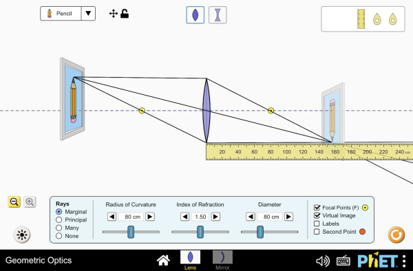
Figure 1:Place a lens or mirror, drag the object, and watch real and virtual images form. This is the interactive companion to the Gaussian imaging constructions later in the chapter.
Interactive simulation: Geometric Optics
1Introduction
Geometrical optics is an old subject, but it is still essential to understand and design optical instruments such as cameras, microscopes, telescopes etc. Geometrical optics started long before light was described as a wave as is done in wave optics, and long before it was discovered that light is an electromagnetic wave and that optics is part of electromagnetism.
In this chapter, we go back in history and treat geometrical optics. That may seem strange now that we have a much more accurate and better theory at our disposal. However, the predictions of geometrical optics are under quite common circumstances very useful and also very accurate. In fact, for many optical systems and practical instruments there is no alternative to geometrical optics because more accurate theories are much too complicated to use.
When a material is illuminated, its molecules start to radiate spherical waves (more precisely, they radiate like tiny electric dipoles) and the total wave scattered by the material is the sum of all these spherical waves. A time-harmonic wave has at every point in space and at every instant of time a well defined phase. A wavefront is a surface of equal phase at a fixed time. In an isotropic medium it moves along its local normal at the phase velocity.
For a plane wave in an isotropic medium, constant-phase surfaces are planes; their normal is the direction of the wave vector and energy flow. A curved wavefront behaves locally like a plane wave when its radius of curvature and the optical features are large compared with the wavelength. Geometrical optics then describes its propagation by rays.
Geometrical optics is based on the intuitive idea that light consists of a bundle of rays. But what is a ray?
Consider a point source at some distance before an opaque screen with an aperture. According to the ray picture, the light distribution on a second screen further away from the source and parallel to the first screen is simply an enlarged copy of the aperture (see Figure 2). The copy is enlarged due to the fanning out of the rays. However, this description is only accurate when the wavelength of the light is very small compared to the diameter of the aperture. If the aperture is only ten times the wavelength, the pattern is much broader due to the bending of the rays around the edge of the aperture. This phenomenon is called diffraction. Diffraction cannot be explained by geometrical optics and will be studied in Scalar Diffraction Optics.
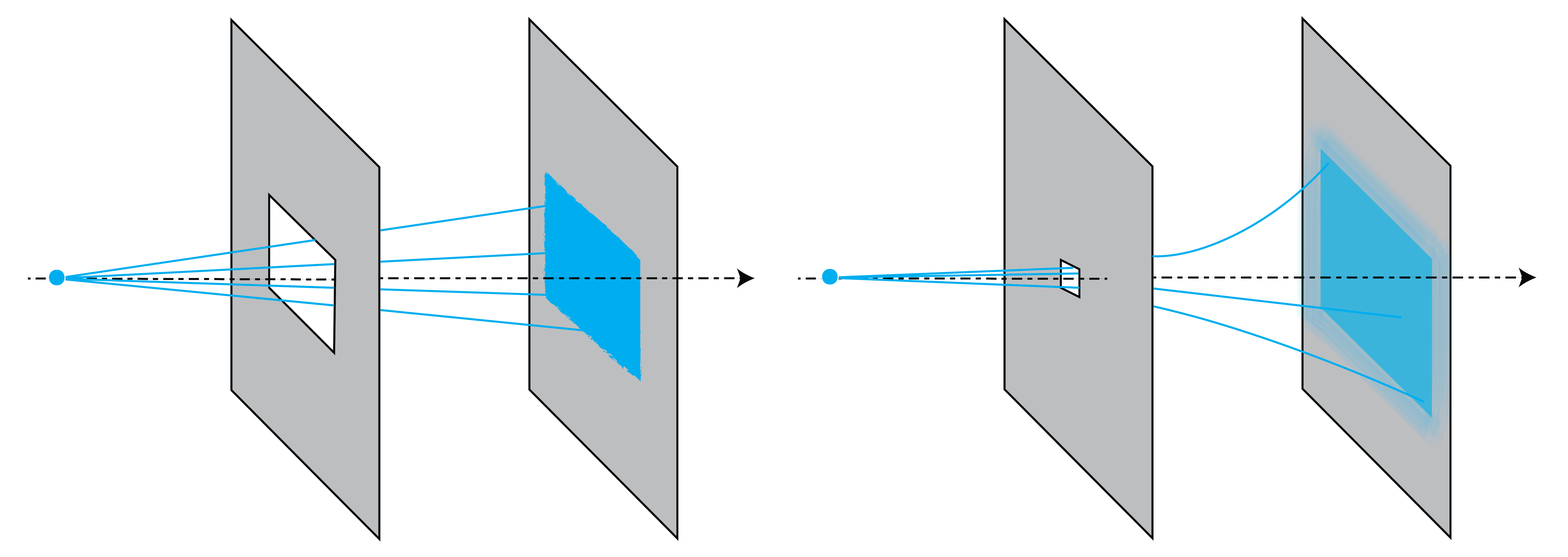
Figure 2:Light distribution on a screen due to a rectangular aperture. Left: for a large aperture, we get an enlarged copy of the aperture. Right: for an aperture that is of the order of the wavelength there is strong bending (diffraction) of the light.
Geometrical optics is accurate when the sizes of the objects in the system are large compared to the wavelength. It is possible to derive geometrical optics from Maxwell’s equations by formally expanding the electromagnetic field in a power series in the wavelength and retaining only the first term of this expansion[1]. However, this derivation is not rigorous because the power series generally does not converge (it is a so-called asymptotic series).
Although it is possible to incorporate polarization into geometrical optics, this is not standard theory and we will not consider polarization effects in this chapter.
2Principle of Fermat
The starting point of the treatment of geometrical optics is the
The phase velocity in a material of refractive index is , where m/s is the vacuum speed. The optical path integral below measures the phase delay at one frequency. In a nondispersive medium this delay equals the ray’s travel time; a pulse in a dispersive medium generally propagates at a different group velocity. Rømer’s 1676 observations of Io’s eclipses established a finite light-travel time.
Let be a ray with the length parameter. The ray links two points and . Suppose that the refractive index varies with position: . Over the infinitesimal distance from to , the speed of the light is
The corresponding differential phase delay, expressed in seconds, is:
The integrated phase delay from to is:
where is the distance along the ray from S to P. The optical path length [m] of the ray between S and P is defined by:
So the OPL is the distance weighted by the refractive index.
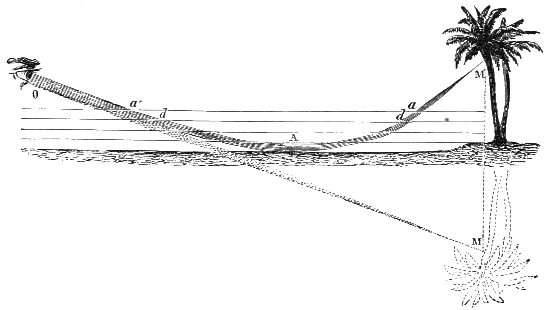
Figure 3:Because the temperature close to the ground is higher, the refractive index is lower there. Therefore the rays bend upwards, creating a mirror image of the tree below the ground. (From Popular Science Monthly Volume 5, Public Domain, link).
Remark. More than one stationary path can connect two points. For example, a direct ray and a reflected ray can have different travel times. The reflection calculation below minimizes travel time among paths constrained to touch the mirror; it does not compare that path with the direct ray.
3Some Consequences of Fermat’s Principle
Homogeneous matter
In homogeneous matter, the refractive index is constant and therefore paths of shortest OPL are straight lines. Hence in homogeneous matter rays are straight lines.
Inhomogeneous matter
When the refractive index is a function of position, as in air with a temperature gradient, the rays bend towards regions of higher refractive index. In the case of Figure 3 for example, on a warm day, the ray from the top of the tree to the eye of the observer passes close to the ground because there the temperature is higher and hence the refractive index is smaller. Although the curved path is longer than the straight path, the total travel time of the light is less because near the ground the light speed is higher (since the refractive index is smaller). The observer gets the impression that the tree is upside down under the ground.
Law of reflection
Consider the mirror shown in Figure 4. In the homogeneous medium above it, a direct ray and a ray reflected by the mirror can connect and . We now minimize travel time over the paths that touch the mirror. Let the -axis be the intersection of the mirror and the plane through the points and and perpendicular to the mirror. Let the -axis be normal to the mirror. Let and be the coordinates of and , respectively. If is the point where a ray from to hits the mirror, the travel time of that ray is
where is the refractive index in . Among paths constrained to reflect at the mirror, the stationary point satisfies
Hence
or
where and are the angles of incidence and reflection as shown in Figure 4.
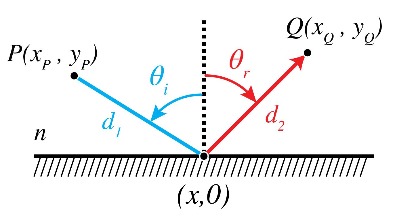
Figure 4:Ray from to via the mirror.
Snell’s law of refraction
Next, we consider refraction at an interface. Let be the interface between a medium with refractive index in and a medium with refractive index in . We use the same coordinate system as in the case of reflection above. Let and with and be the coordinates of two points and as shown in Figure 5. What path will a ray follow that goes from to ? Since the refractive index is constant in both half spaces, the ray is a straight line in both media. Let be the coordinate of the intersection point of the ray with the interface. Then the travel time is
The OPL is stationary with respect to the crossing point, so
where the phase delay has been multiplied by the vacuum light speed. Eq. (10) implies
where and are the angles between the ray and the normal to the surface in the upper half space and the lower half space, respectively (Figure 5).
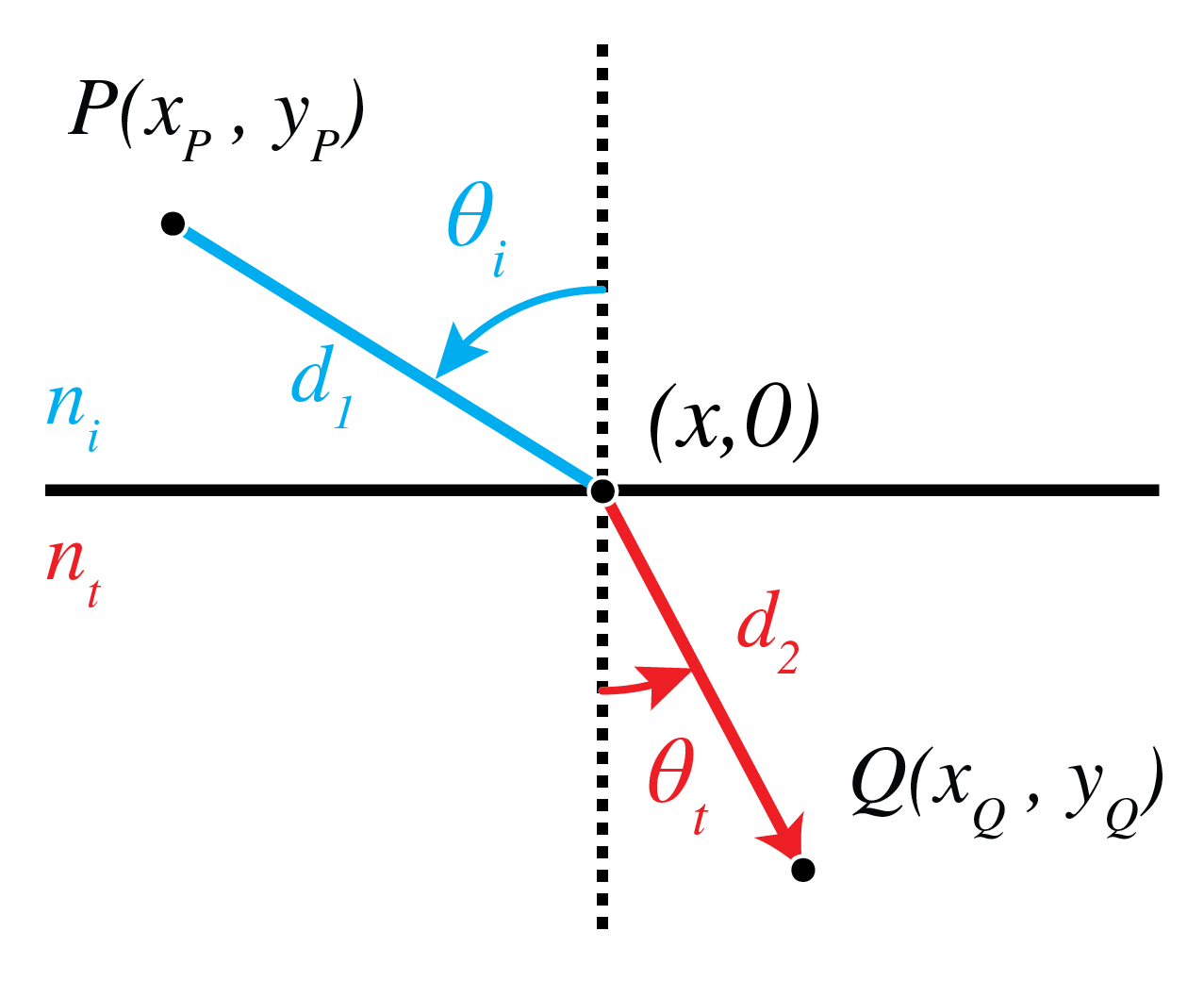
Figure 5:Ray from to refracted by an interface.
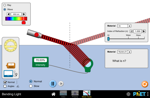
Figure 6:Refraction and reflection at a planar interface with adjustable indices. Measure and and check that matches the protractor — the same Snell’s law just derived from Fermat’s principle.
Interactive simulation: Bending Light
Thus Fermat’s principle gives the reflection and refraction laws. Matching the phase of electromagnetic fields along an interface gives an independent derivation of Snell’s law.
4Perfect Imaging by Conic Sections
In this section, the conic sections ellipse, hyperbola and parabola are important. In Figure 8 their definitions are shown as a quick reminder[3].
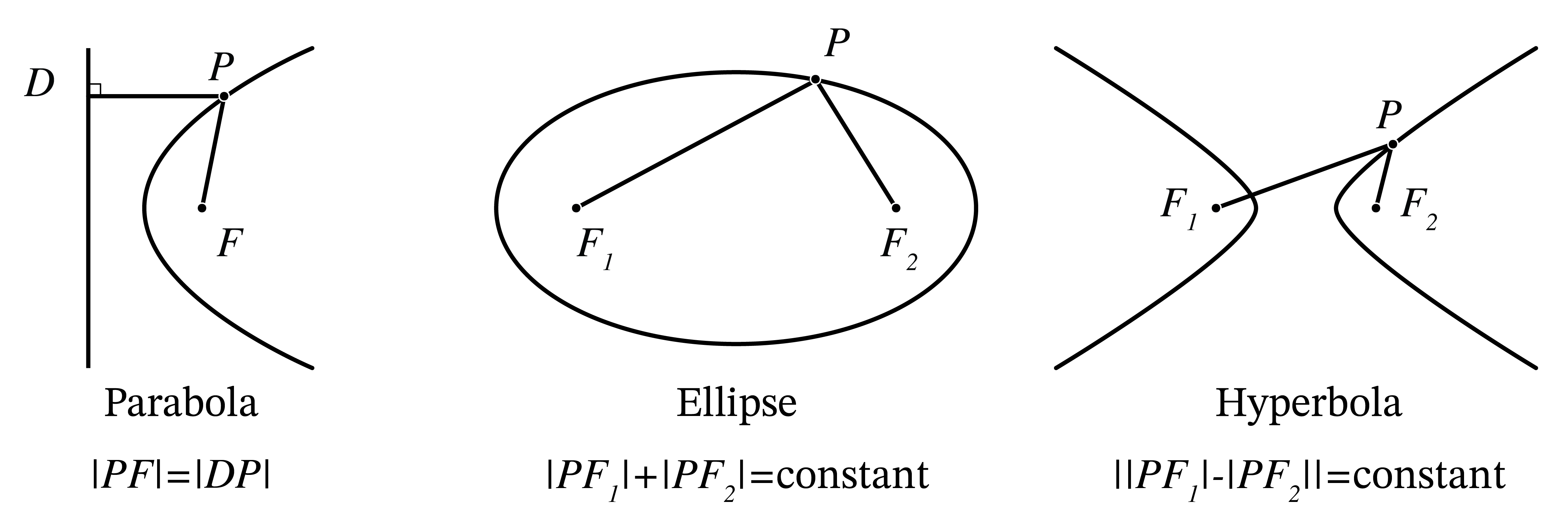
Geometric construction of conic sections (ellipse, hyperbola, and parabola) showing their traditional definitions. The ellipse is the locus of points with constant sum of distances to two foci, the hyperbola has a constant difference of distances, and the parabola maintains equal distances to a focus and a directrix.
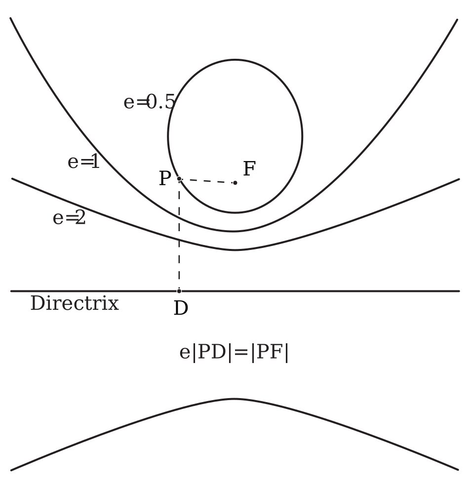
Figure 8:Conic sections through the focus–directrix relation : gives an ellipse, a parabola, and a hyperbola. The horizontal line through is the common directrix in this drawing.
We start by explaining what in geometrical optics is meant by perfect imaging. Let be a point source. The rays perpendicular to the spherical wave fronts emitted by radially fan out from . Due to objects such as lenses etc. the spherical wave fronts are deformed and the directions of the rays are made to deviate from the radial propagation direction. If every ray in a cone from meets again at , as in Figure 9, is a perfect geometrical image of . For an ideal stigmatic system, the wavefront arriving at also has equal optical phase across the contributing aperture. Fermat’s stationarity condition alone does not say that arbitrary rays have equal travel times. By reversing the direction of the rays, is similarly a perfect image of . The optical system in which this happens is called stigmatic for the two points and .
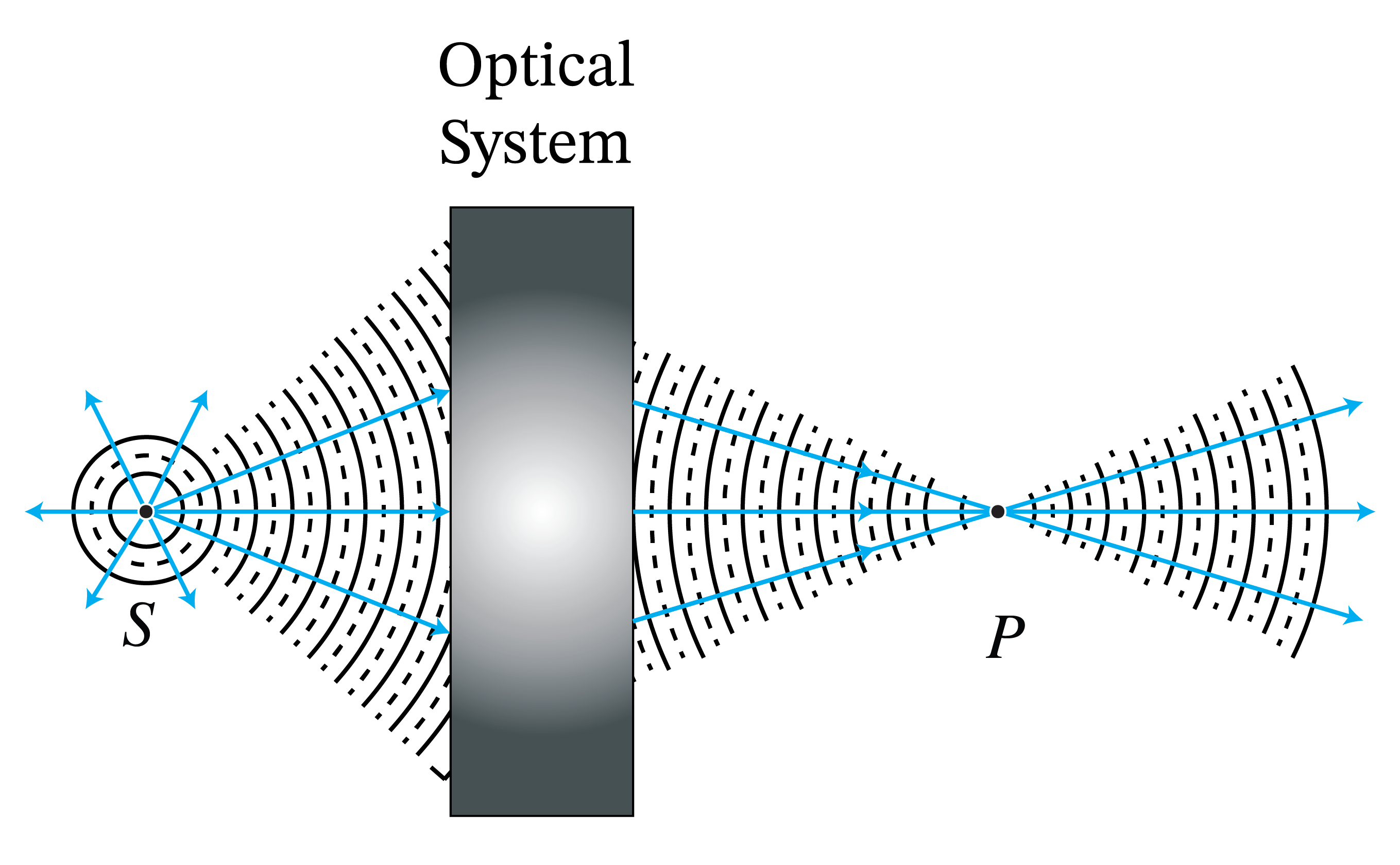
Figure 9:Perfect imaging: a cone of rays which diverge from and all intersect in point . The rays continue after .
Remark. The concept of a perfect image point exists only in geometrical optics. In reality, finite apertures of lenses and other imaging systems cause diffraction due to which image points are never perfect but blurred.
We summarize the main examples of stigmatic systems.
1. Perfect focusing and imaging by refraction. A parallel bundle of rays propagating in a medium with refractive index can be focused into a point in a medium with refractive index . If , the interface between the media should be a hyperbola with focus , whereas if the interface should be an ellipse with focus . By reversing the rays we obtain perfect collimation. Therefore, a point in air can be perfectly imaged onto a point in air by inserting a piece of glass in between them with hyperbolic surfaces. These properties are derived in Problem 2.2.
2. Perfect focusing of parallel rays by a mirror. A bundle of parallel rays in air can be focused into a point by a mirror of parabolic shape with as focus. This is derived in Problem 2.3. By reversing the arrows, we get (within geometrical optics) a perfectly parallel beam. Parabolic mirrors are used everywhere, from automobile headlights to radio telescopes.
Remark.
Although we found that conic surfaces give perfect imaging for a certain pair of points, other points do not have perfect images in the sense that for a certain cone of rays, all rays are refracted (or reflected) to the same point.
5Gaussian Geometrical Optics
We have seen that, although by using lenses or mirrors which have surfaces that are conic sections we can perfectly image a certain pair of points, for other points the image is not perfect. The imperfections are caused by rays that make larger angles with the optical axis, i.e. with the symmetry axis of the system. Rays for which these angles are small are called paraxial rays. Because for paraxial rays the angles of incidence and transmission at the surfaces of the lenses are small, the sines of the angles in Snell’s Law are replaced by the angles themselves:
This approximation greatly simplifies the calculations. At first paraxial order, a smooth rotationally symmetric surface can be replaced by a sphere with the same curvature at its vertex. Higher-order terms determine its aberrations outside that approximation. Spherical surfaces are not only simpler in the derivations but they are also much easier to manufacture. Hence in the optical industry spherical surfaces are used a lot. To reduce imaging errors caused by non-paraxial rays one applies two strategies: 1. adding more spherical surfaces; 2. replacing one of the spherical surfaces (typically the last before image space) by a non-sphere.
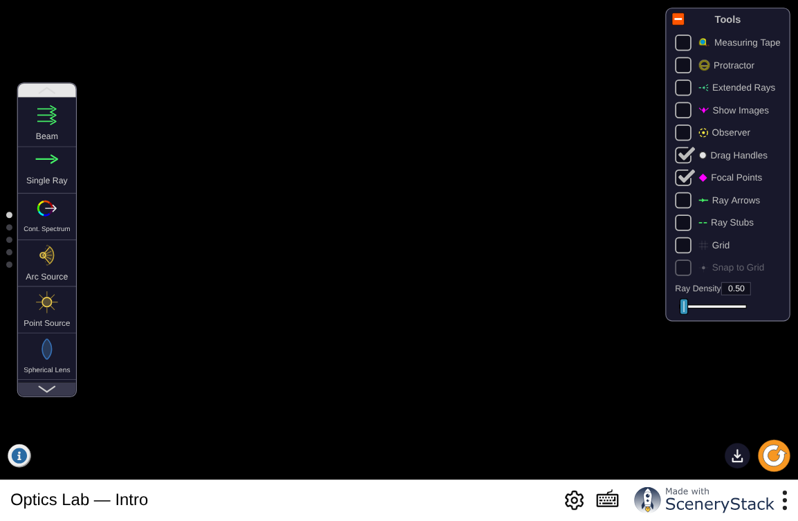
Figure 10:An open optical bench: rays, parallel and divergent beams, lenses, mirrors, and refracting interfaces. Build the single-surface and thin-lens geometries of this section and watch where the rays meet.
Interactive simulation: Optics Lab
5.1Gaussian Imaging by a Single Spherical Surface
We will first show that within Gaussian optics a single spherical surface between two media with refractive indices images all points perfectly (Figure 11). The sphere has radius and center which is inside medium 2. We consider a point object to the left of the surface. We draw a ray from perpendicular to the surface. The point of intersection is . Since for this ray the angle of incidence with the local normal on the surface vanishes, the ray continues into the second medium without refraction and passes through the center of the sphere. Next we draw a ray that hits the spherical surface at some point and draw the refracted ray in medium 2 using Snell’s law in the paraxial form Eq. (12). Note that the angles of incidence and transmission must be measured with respect to the local normal at , i.e. with respect to . We assume that this ray intersects the first ray at point . We will show that within the approximation of Gaussian geometrical optics, all rays from pass through . Furthermore, with respect to a coordinate system with origin at , the -axis pointing from to and the -axis positive upwards as shown in Figure 11, we have:
where
is called the power of the surface and where and are the -coordinates of and , respectively, hence and in Figure 11.
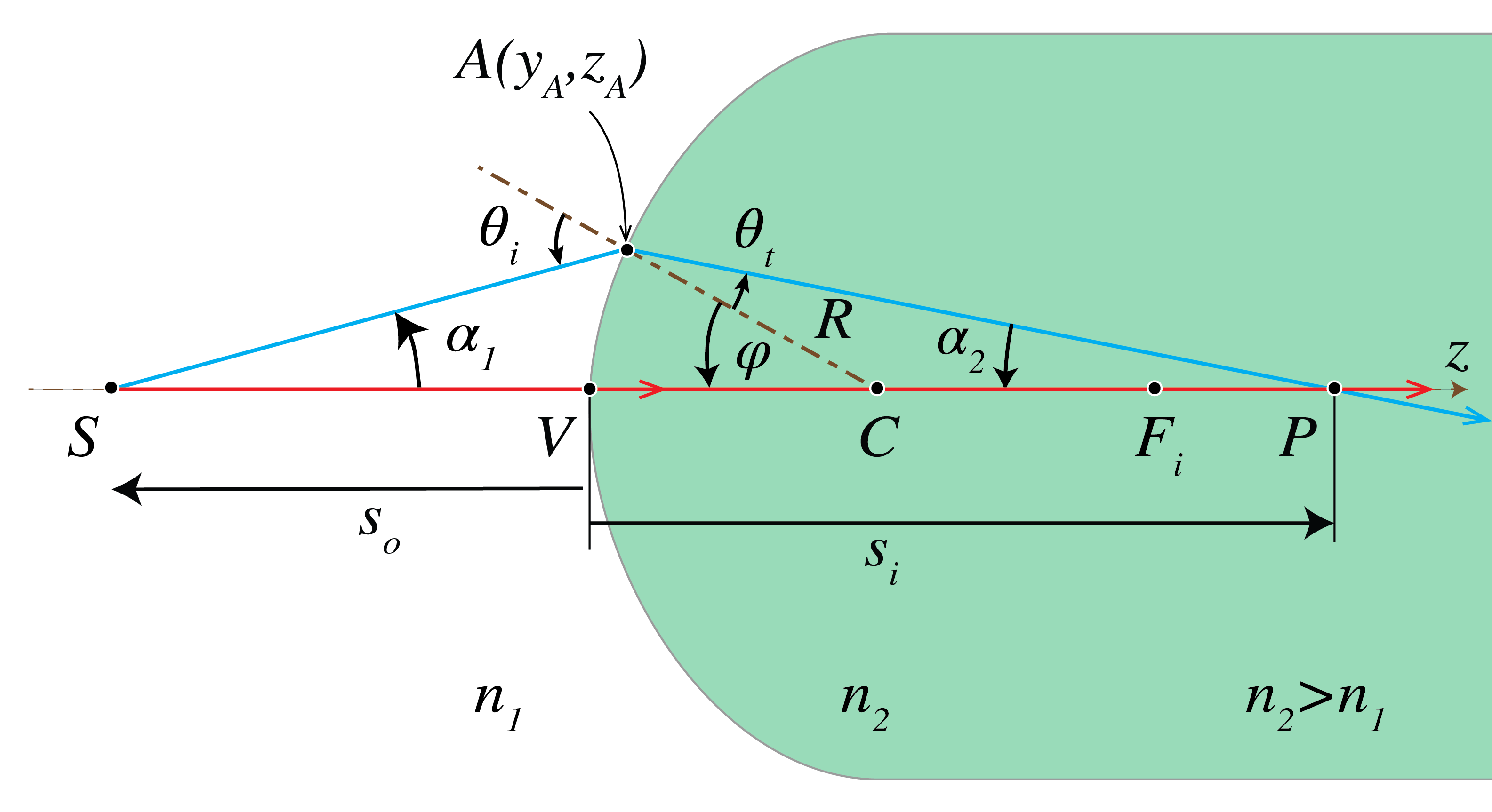
Figure 11:Imaging by a spherical interface between two media with refractive indices .
Proof.
It suffices to show that is independent of the ray, i.e. of . We will do this by expressing in terms of and showing that the result is independent of . Let and be the angles of the rays and with the -axis as shown in Figure 11. Let be the angle of incidence of ray with the local normal on the surface and be the angle of refraction. By considering the angles in triangle we find
Similarly, from we find
By substitution into the paraxial version of Snell’s Law Eq. (12), we obtain
Let and be the coordinates of point . Since and we have
Furthermore,
which is small for paraxial rays. Hence,
because it is second order in and therefore is neglected in the paraxial approximation. Then, Eq. (18) becomes
By substituting Eq. (21) and Eq. (19) into Eq. (17) we find
or
which is Eq. (13). It implies that , and hence , is independent of , i.e. of the ray chosen. Therefore, is a perfect image within the approximation of Gaussian geometrical optics.
When , the incident rays are parallel to the -axis in medium 1 and the corresponding image point is called the second focal point or image focal point. Its -coordinate is given by:
The absolute value of is called the second focal length or image focal length. For , the signed value is negative when . When , the rays after refraction are parallel to the -axis and we get . The object point for which the rays in medium 2 are parallel to the -axis is called the first focal point or object focal point . Its -coordinate is:
The absolute value of is called the front focal length or object focal length.
With Eq. (24) and Eq. (25), Eq. (13) can be rewritten as:
5.2Virtual Images and Virtual Objects of a Single Spherical Surface
If we adopt the sign convention listed in Table 1 below, it turns out that Eq. (13) holds generally. So far we have considered a convex surface of which the center is to the right of the surface, but Eq. (13) applies also to a concave surface of which the center is to the left of the surface, provided that the radius is chosen negative. The convention for the sign of the radius is illustrated in Figure 12.
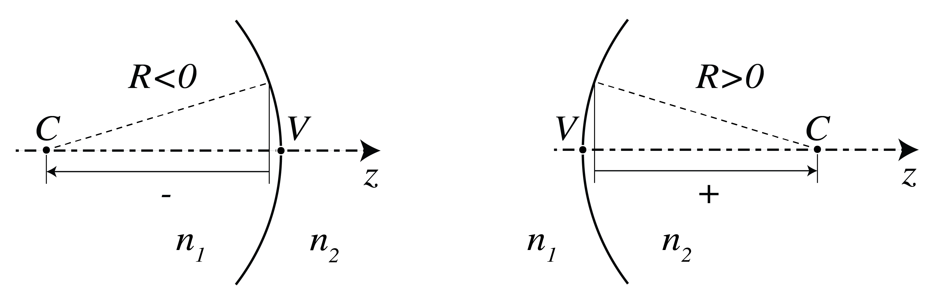
Figure 12:Sign convention for the radius of a spherical surface
If the power given by Eq. (14) is positive, then the surface makes bundles of incident rays convergent or less divergent. If the power is negative, incident bundles are made divergent or less convergent. The power of the surface can be negative for two reasons:
>0 and , or
<0 and , but the effect of the two cases is the same. For any object to the left of the surface: , Eq. (26) and a negative power imply that , which suggests that the image is to the left of the surface. Indeed, in both cases, the diverging ray bundle emitted by S is made more strongly divergent by the surface. By extending these rays in image space back to object space (without refraction at the surface), they are seen to intersect in a point to the left of the surface. This implies that for an observer at the right of the surface it looks as if the diverging rays in image space are emitted by . Because there is no actual concentration of light intensity at , it is called a virtual image, in contrast with the real images that occur to the right of the surface and where there is an actual concentration of light energy. We have in this case and , which means that the object and image focal points are to the right and left, respectively, of the surface.
Note that also when the power is positive, a virtual image can occur, namely when the object is in between the object focal point and the surface. Then the bundle of rays from S is so strongly diverging that the surface cannot convert it into a convergent bundle and hence again the rays in image space seem to come from a point to the left of the surface. This agrees with the fact that when and , Eq. (26) implies that .
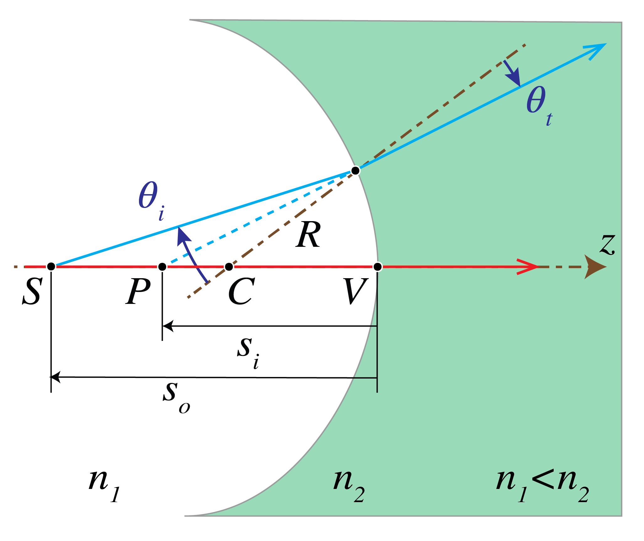
Figure 13:Imaging by a concave surface () with . All image points are to the left of the surface, i.e. are virtual ().
Finally we look at a case in which there is a bundle of convergent rays incident on the surface from the left. If extended into the right medium without refraction, these rays would intersect in a point . Since this point is not actually present, it is called a virtual object point, in contrast to real object points which are to the left of the surface. The coordinate of a virtual object point is positive: . One may wonder why we look at this case. The reason is that if we have several spherical surfaces behind each other, we can compute the image of an object point by first determining the intermediate image by the leftmost surface and then use this intermediate image as the object for the next surface and so on. In such a case, it can easily happen that an intermediate image is to the right of the next surface and hence is a virtual object for that surface. In the case of Figure 14 at the left, the power is positive, hence the convergent bundle of incident rays is made even more convergent which leads to a real image point. Indeed when and then Eq. (13) implies that always . At the right of Figure 14 the power is negative but is not sufficiently strong to turn the convergent incident bundle into a divergent bundle. So the image is still real. However, the image will be virtual when the virtual object is to the right of (which in this case is to the right of the surface) since then the bundle of rays converges so weakly that the surface turns it into a divergent bundle.
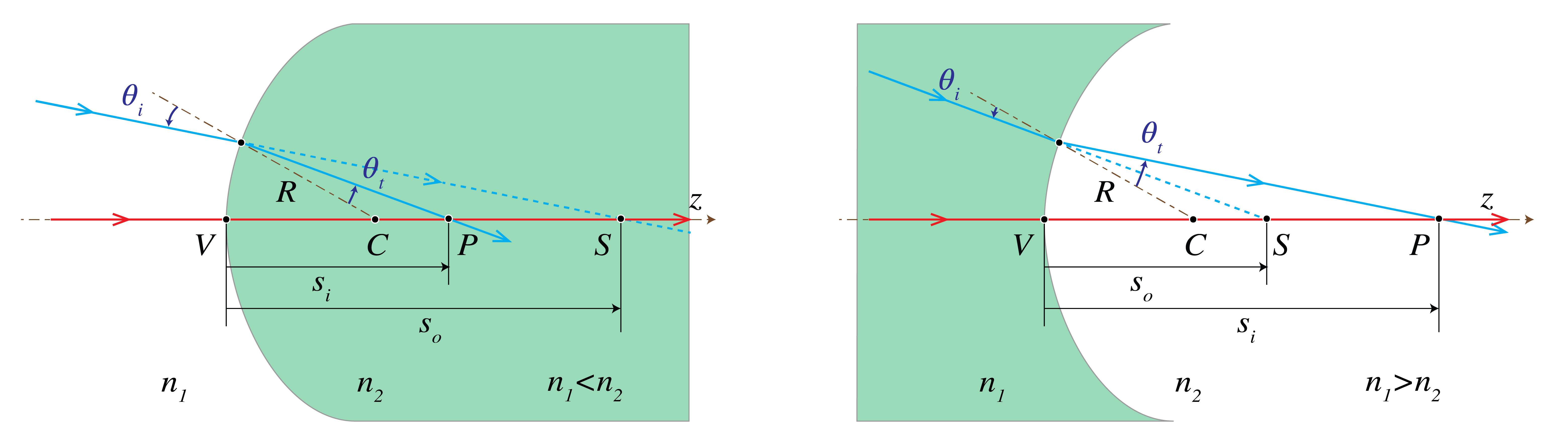
Figure 14:Imaging of a virtual object by a spherical interface with between two media with refractive indices (left) and (right).
In conclusion: provided the sign convention listed in Table 1 is used, formula Eq. (13) can always be used to determine the image of a given object by a spherical surface.
The convention for , , , follows from the fact that these are -coordinates with the origin at vertex of the spherical surface (or the center of the thin lens) and the positive -axis is pointing to the right. The convention for the -coordinate follows from the fact that the -axis is positive upwards.
Table 1:Sign convention for spherical surfaces and thin lenses
| quantity | positive | negative |
|---|---|---|
| , , , | corresponding point is to the right of vertex | corresponding point is to the left of vertex |
| , | object, image point above optical axis | object, image point below optical axis |
| center of curvature right of vertex | center of curvature left of vertex |
5.3Stops
An element such as the rim of a lens or a diaphragm which determines the set of rays that can contribute to the image is called the aperture stop. An ordinary camera has a variable diaphragm.
The entrance pupil is the image of the aperture stop by all elements to the left of the aperture stop. In constructing the entrance pupil, rays are used which propagate from the right to the left. The image can be real or virtual. If there are no lenses between object and aperture stop, the aperture stop itself is the entrance pupil. Similarly, the exit pupil is the image of the aperture stop by all elements to the right of it. This image can be real or virtual. The entrance pupil determines for a given object the cone of rays in object space that contribute to the image, while the cone of rays leaving the exit pupil is the one taking part in image formation (see Figure 15).
For any object point, the chief ray is the ray in the cone that passes through the center of the entrance pupil, and hence also through the centers of the aperture stop and the exit pupil. A marginal ray is the ray that for an object point on the optical axis passes through the rim of the entrance pupil (and hence also through the rims of the aperture stop and the exit pupil).
The entrance pupil controls the cone of light accepted from an object point. For a camera focused on a distant scene, the nominal -number is the effective focal length divided by the entrance-pupil diameter :
For example, means . At the same transmission and scene conditions, irradiance is approximately inversely proportional to the square of the -number, so needs about half the exposure time of . Finite-distance imaging and transmission losses can modify this simple comparison.
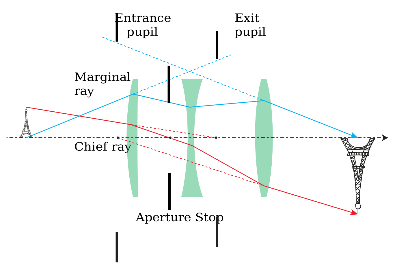
Figure 15:Aperture stop between the first and second lenses. The entrance pupil is the stop’s image seen from object space, and the exit pupil is its image seen from image space. The chief and marginal rays are shown.
6Beyond Gaussian Geometrical Optics
6.1Aberrations
For designing advanced optical systems Gaussian geometrical optics is not sufficient. Instead non-paraxial rays, and among them also non-meridional rays, must be traced using software based on Snell’s Law with the sine of the angles of incidence and refraction. Often many thousands of rays are traced to evaluate the quality of an image. It is then found that in general the non-paraxial rays do not intersect at the ideal Gaussian image point. Instead of a single spot, a spot diagram is found which is more or less confined. The deviation from an ideal point image is quantified in terms of aberrations. One distinguishes between monochromatic and chromatic aberrations. The latter are caused by the fact that the refractive index depends on wavelength. Recall that in paraxial geometrical optics Snell’s Law Eq. (11) is replaced by: , i.e. and are replaced by the linear terms. If instead one retains the first two terms of the Taylor series of the sine, the errors in the image can be quantified by five monochromatic primary (Seidel) aberrations. The best known is spherical aberration, which is caused by the fact that for a convergent spherical lens, the rays that make a large angle with the optical axis are focused closer to the lens than the paraxial rays (see Figure 16).
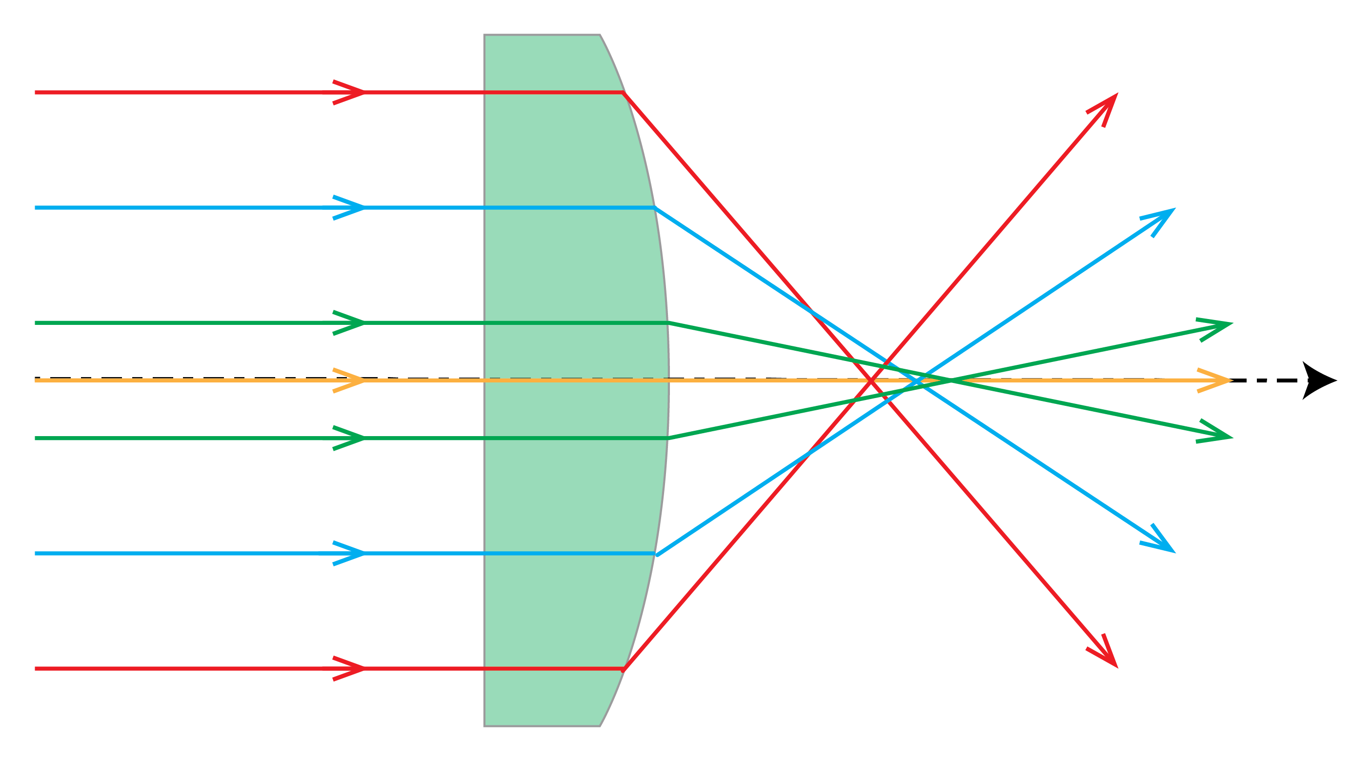
Figure 16:Spherical aberration of a planar-convex lens.
Distortion is one of the five primary aberrations. It causes deformation of images due to the fact that the magnification depends on the distance of the object point to the optical axis.
For high-quality imaging, the aberrations have to be reduced by adding more lenses and optimizing the curvatures of the surfaces, the thicknesses of the lenses and the distances between them. For high-quality systems, a lens with an aspherical surface is sometimes used. Systems with very small aberrations are extremely expensive, in particular if the field of view is large, as is the case in lithographic imaging systems used in the manufacturing of integrated circuits as illustrated by the lithographic system in Figure 17.
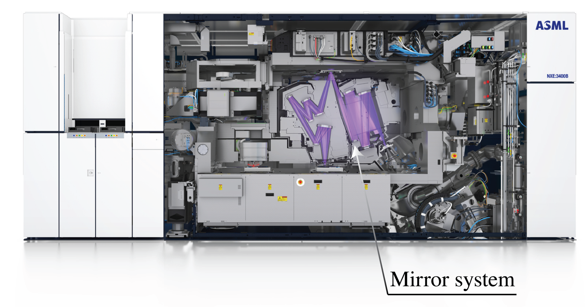
Figure 17:ASML’s TWINSCAN NXE:3400B extreme-ultraviolet lithography system. The purple overlay traces its reflective projection optics; EUV systems use 13.5 nm light and mirrors rather than transmissive lenses (ASML product information).
6.2Diffraction
According to a generally accepted criterion formulated first by Rayleigh, aberrations start to deteriorate images considerably if they cause path length differences of more than a quarter of the wavelength. When the aberrations are less than this, the system is called diffraction limited.
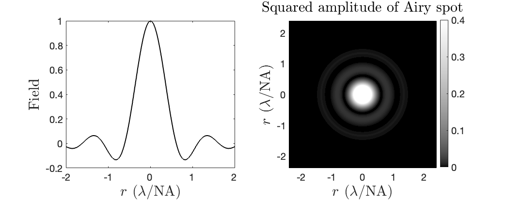
Figure 18:Left: cross section of the field of the Airy pattern. Right: intensity pattern of the Airy pattern.
Even if the wave transmitted by the exit pupil were perfectly spherical (no aberrations), its finite aperture causes diffraction. A point object therefore forms an Airy pattern rather than a point (Figure 18). For an ideal uniformly illuminated circular pupil, the central intensity spot has approximate full width at half maximum:
where is the vacuum wavelength and is the image-space numerical aperture. Here is the half-angle of the cone from the exit pupil to the image point; in air and the paraxial limit, for exit-pupil radius and distance from that pupil to the image. Diffraction depends on wavelength and therefore lies beyond pure geometrical optics. We treat aperture diffraction in Scalar Diffraction Optics.
7Chapter Summary
Fermat’s principle makes optical path length stationary under small changes to a ray path.
In Gaussian geometrical optics, the paraxial (small angle) approximation enables analytical treatment of imaging by spherical surfaces.
For a single spherical interface, with the signed coordinates used here.
Real images form where rays converge; virtual images form where rays appear to originate.
Spherical aberration limits imaging quality for rays far from the optical axis; it can be minimized using aspherical surfaces or conic sections.
Stops and pupils: The aperture stop limits the light cone; entrance and exit pupils are its images as seen from object and image space.
The -number is effective focal length divided by entrance-pupil diameter.
Geometrical optics breaks down when feature sizes approach the wavelength, leading to diffraction effects described by the Airy pattern.