Photo credit: Tom Murphy
12. Wind Energy
Wind energy has made significant inroads for electricity production in the U.S. and globally. Today, the U.S. gets about 2.5% of its energy (and 6.5% of electricity) from wind. Globally, wind accounts for about 2.6% of energy, or 4.8% of electrical production (Table 7.2; p. 112).
The basic technology of harnessing wind power is rather old, powering ships, milling operations, and water pumps for centuries. Today, the predominant use of wind drives generators to make electricity.
Just as hydroelectric power is related to the very basic form of gravitational potential energy, wind is connected to another simple and easy-to-understand form: kinetic energy. This chapter first develops familiarity with kinetic energy, then explores how we get energy from wind, how much we get, and future prospects.
12.1 Kinetic Energy
An object in motion carries kinetic energy equal to one-half its mass times the velocity squared.
Often, we use energy sources to deliver kinetic energy, as in moving planes, trains and automobiles.
But we can also go the other direction and convert kinetic energy into different forms of energy[3] for versatile use. Most commonly, we turn kinetic energy into electrical potential energy (a voltage) that can drive a circuit. At this point, the energy can be used to toast a bagel, charge a phone, or wash clothes.
The method for converting kinetic energy into electricity is usually accomplished by transferring kinetic energy in a moving fluid[4] into rotation of a shaft by way of a turbine—essentially fan blades. The spinning shaft then turns an electric generator, which consists of the relative motion between magnets and coils of wire, and is essentially the same construction/concept as an electric motor run in reverse.
Hydroelectric installations do the same thing—turning a shaft via blades of a turbine—even though we framed the energy source as one of gravitational potential energy. Within the dam’s turbine, the water acquires kinetic energy as it flows from the reservoir to the outlet. Wind energy acts in much the same way, converting kinetic energy in the moving air into rotational motion of a fan/turbine whose shaft is connected to a generator located behind the blades.
12.2 Wind Energy
It is tempting to think of air as “empty” space, but at sea level air has a density of 1.25 kg per cubic meter . Let this sink in visually: imagine a cubic meter sitting next to you (as in Figure 12.1). The air within has a mass of 1.25 kg (about 2.75 lb). Now draw a square meter on the ground—either literally or in your imagination. The many kilometers of air extending vertically over the top of that square meter has a mass of kg! For context, figure out how many cars that would be (typ. 1,500 kg ea.), or what kind of animal would be this massive.
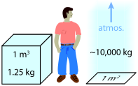
Figure 12.1:The mass of a cubic meter of air is 1.25 kg, and the mass of atmosphere over one square meter is an astounding 10 metric tons.
What this means is that air in motion can carry a significant amount of kinetic energy, since neither its mass nor velocity are zero. If the entire earth’s atmosphere moved at 5 m/s—a noticeable breeze—at a total mass[5] of 5 kg, we’d have 6 J of kinetic energy in air currents. If we somehow pulled all this energy out of the air—stopping its motion entirely—we might expect the atmosphere to revive its normal wind
patterns over the course of 24 hours: a full day of the driving solar input around the globe. The associated power works out to 700 TW. Notice that the value for wind in Table 10.2 (p. 175) is pretty-darned close to this, at 900 TW.[6] As the margin note indicates, we should be pleased to get within a factor of two for so little work and very off-the-cuffassumptions about global average air speed (see Box 12.1 for related thoughts). Figure 12.2 shows the annual average wind velocity at a height of 80 m (typical wind turbine height) for the U.S. Note that the 5 m/s we used above falls comfortably within the 4–8 m/s range seen in the map.
![Average wind velocity at a height of 80 m across the U.S. [69]. Boundaries between colored boxes are every 0.5 m/s from 4.0 m/s to 10.0 m/s.](/EnergyAndHumanAmbitions/build/fig-12-2-352265daac85eb6b441a2ab79d4f3c8f.png)
Figure 12.2:Average wind velocity at a height of 80 m across the U.S. [69]. Boundaries between colored boxes are every 0.5 m/s from 4.0 m/s to 10.0 m/s. Nothing on this map exceeds 9 m/s, and the deepest green is below 4 m/s. The plains states are the hot ticket. Note that Alaska is not to scale. From NREL.
But we can’t capture the entire atmospheric wind, because doing so would require wind turbines throughout the volume, up to 10 km high! In fact, some estimates [70] of practical global wind installations come in as low as 1 TW—well below our 18 TW demand. Wind alone is unlikely
able to replace the energy currently derived from fossil fuels.
12.2.1 Wind Turbines
To understand practically-available energy, we back up and consider how much air hits a wind turbine whose rotor diameter is . Figure 12.3 illustrates the concept. If the wind speed is , the air travels a distance in time interval .[9]
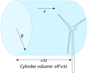
Figure 12.3:Wind power concept. In time interval at wind speed , a volume of air encounters the rotor having the shape of a cylinder of radius and length . Note that most wind turbines are designed to pivot about a vertical axis to face into the wind, whatever the direction.
The cross-sectional area of the wind turbine (rotor) is defined as the area swept out by the blades, so . Thus the volume of the cylinder of air interacting with the turbine over time interval is the “base” (circular) area of the cylinder times its “height” (straight length, , or . We know the density of the air,[10] so the mass of the cylinder is . The kinetic energy contained in this cylinder of air is therefore . Now let’s get rid of that pesky . Think for a moment what happens if we divide both sides by : it will definitely get rid of the on the right-hand-side, but what does the left-hand side mean: energy over time? Hopefully, this is familiar by now as the concept of power.
Table 12.1:Wind power scales as the cube of wind speed.
| Speed | Power |
|---|---|
| 0 | 0 |
| 1 | 1 |
| 2 | 8 |
| 3 | 27 |
| 4 | 64 |
| 5 | 125 |
| ⋮ | ⋮ |
| 10 | 1,000 |
Notice that the delivered power scales, sensibly, with the area of the wind turbine’s blade path, but more importantly and perhaps surprisingly as the velocity cubed (Table 12.1). The cubed part should make you sit up straight: that’s a very strong function of velocity! It means that if the wind changes from a gentle 5 m/s to a brisk 10 m/s, the power available goes up by a factor of 8. A strong wind at 20 m/s has 64 times as much power as the 5 m/s breeze.[11] We can understand the three powers of velocity thusly: two powers come from kinetic energy, and one from the length of the cylinder. As wind speed increases, not only does the oncoming air have more kinetic energy per fixed volume, but also a larger volume encounters the turbine in a given time.
Setting in Eq. 12.2 corresponds to the total power present in the wind. But we can’t be greedy and grab all of it. In fact, if we did, it would mean stopping the air at the wind turbine: pulling out all the kinetic energy means no velocity is left. If we did this, newly arriving air would divert around the stopped mass of air, and the turbine would no longer have access to oncoming energy. The theory has all been worked out:[12] a turbine is limited to (59%) of the available energy, known as the Betz limit [72]. This is not a technological limitation, but comes from the physics of fluid flow. A second consideration enters for low-speed rotor motion, known as the Glauert limit [73], resulting in diminishing efficiency as wind speed drops.
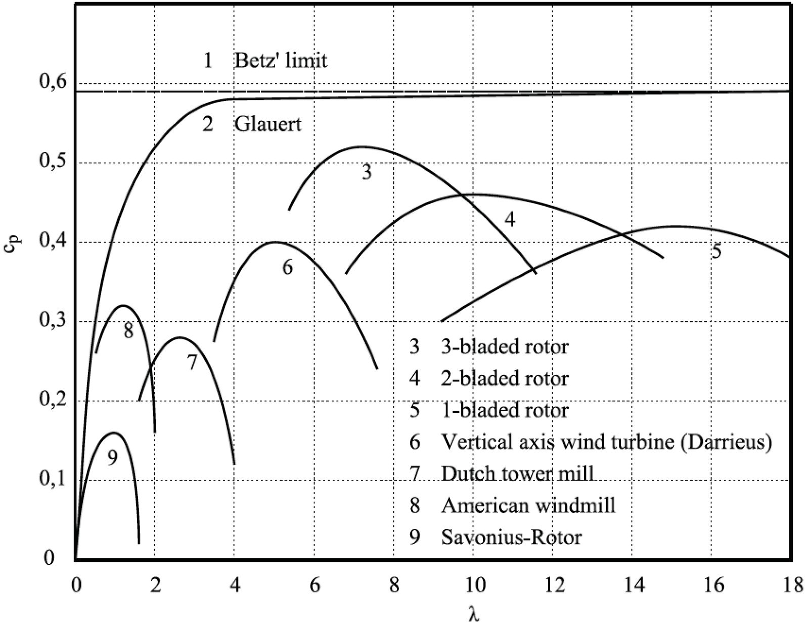
Figure 12.4:Theoretical and practical wind turbine efficiencies , or c in the plot), for various designs. The parameter is the ratio of tip speed to wind speed: higher means a faster tip speed [74]. All designs must be below the Betz limit (horizontal line near top). At slower speeds, the Glauert limit confines performance to occupy the region to the right of the curve marked 2. Each of the 7 designs shown have arched curves, achieving maximum efficiency at a particular tip speed. Too slow, and the turbine is not transmitting much energy; too fast and drag/friction begins to dominate. Adapted from ©2010 WIT Press.
Figure 12.4 shows these theoretical limits, along with design limits from various rotor configurations. Curves reflect an optimum rotor speed for each design: speeding up produces more generator output until it gets fast enough that air drag on the blades starts to dominate. The most common modern turbine is the 3-blade design,[13] able to get roughly 50% of the energy out of the wind. Notice that the tip speed can be quite high: 6–8 times the wind speed. This can be quite alarming to birds in the area, whose cruising speed is nearer wind speed, and they
have never met something so fast before. For a modern derivation of the Betz limit and how efficiency depends on tip speed, see [71]. The largest turbines—having 150 m diameter rotors—are rated for up to 10 MW of electrical power production.
Besides the limit on how much power can be pulled out of the air by a single turbine, we also find limits on how densely they may be populated in a given area: how much space is required between turbines so that one does not disrupt the other. Obviously, it would not serve to put one turbine directly behind another, as they would at best split the available power arriving as wind. Even side by side, it is best to leave room between windmills so that additional rows are not deprived of wind power. A rule of thumb is to separate turbines by at least 5–8 diameters side-to-side, and 7–15 diameters[15] along the (prevailing) wind direction. For the sake of illustration, Figure 12.5 shows a spacing on the denser side of the range, but otherwise we adopt the more recent recommendations and use 8 diameters side-to-side and 15 diameters deep [75]. This works out to a 0.65% “fill factor,” meaning that 0.65% of the land area contains an associated rotor cross section.[16]
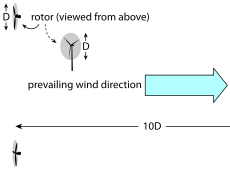
Figure 12.5:Overhead view of wind farm turbine locations, for the case where separations are 10 rotor-diameters along the wind direction, and 5 rotor diameters in the cross-wind direction—a geometry that yields 1.6% area “fill factor.” Current recommendations are for 15 and 8 rotor diameters, which is significantly more sparse than even this depiction, leading to 0.65% area fill. Note that most wind turbines can turn to face the wind direction, for times when its direction is not the prevailing one.
5D
In order to compare to other forms of renewable energy, we can evaluate a power per unit land area (in by the following approach:
employing the rule-of-thumb 8 turbine placement scheme. Using an efficiency of 40% and m/s,[17] we get 0.2 —which is 1,000 times smaller than solar’s insolation (Ex. 10.3.1; p. 174).
A final general note about wind generation is somewhat obvious: the wind is not always blowing, and its speed varies over wide ranges. In this sense, wind is an intermittent power source. Just as for hydroelectric installations, wind resources are characterized by a regionally-dependent capacity factor, which is the ratio of energy delivered to what would have been delivered if the generation facility operated at full capacity at all times. Typical capacity factors for wind in the U.S.[18] are around 33%, and Figure 12.6 provides a visual sense for how this manifests in the real world: pretty erratic.
![One month of wind generation from a 20 MW wind farm, illustrating the intermittent nature and why capacity factors are low [76]. The facilit](/EnergyAndHumanAmbitions/build/fig-12-6-0b5193fc98d13da18e5daa5ec7499e5d.jpg)
Figure 12.6:One month of wind generation from a 20 MW wind farm, illustrating the intermittent nature and why capacity factors are low [76]. The facility saturates at maximum power late in the month, self-limiting to avoid damage to the turbines. ©2010 Springer.
For very low wind speeds,[19] wind turbines do not have enough wind to turn at all and sit still at zero output. Furthermore, a turbine is rated at some maximum power output, which occurs at some moderately high wind speed,[20] beyond which the generator risks damage—like “redlining” a car’s engine. When the wind climbs above this maximum-rated speed, the turbine is pegged at its maximum power—no longer following a relation—and deliberately twists its blades[21] to be less efficient as the wind speed grows so that it maintains constant (maximum) power output. When the wind speed becomes large enough to endanger the turbine, it will twist its blades parallel to the wind to allow the air to pass without turning the rotor at all, so that it no longer spins while it “rides out” the high winds.[22]
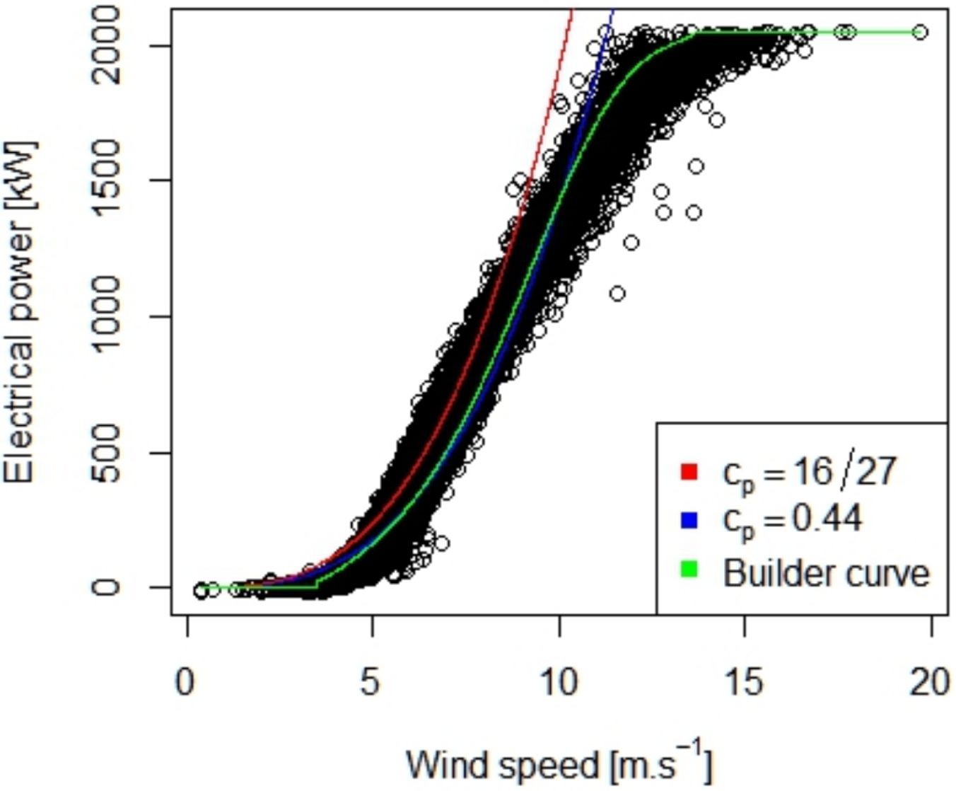
Figure 12.7:Actual data (thickly-clustered black circles) of power delivered by a turbine rated at 2 MW, as a function of wind velocity. The red curve represents the theoretical Betz limit of 59%, appearing as a cubic function of velocity—as Eq. 12.2 dictates. The better-matching blue curve corresponds to an overall efficiency c (44%), and the green curve—which rolls over from the cubic function and saturates at higher velocities—is the manufacturer’s expectation for the unit [77]. The “cut-in” velocity for this turbine is around 3.5 m/s: note the small step up from zero output in the green curve. This turbine saturates around 12 m/s: the green curve flattens out and no black circles appear above the cutoff. From ©2017 Wiley.
Figure 12.7 shows a typical power curve for a 2 MW turbine, on top of which are drawn a cubic function of velocity at the theoretical Betz limit (red curve), a cubic (blue) at 44% efficiency , and the green manufacturer’s curve [77]. Notice that the turbine performance
demonstrates the aspects covered in the previous paragraph: “cutting in” just above 3 m/s and maxing out (saturating) beyond about 12 m/s. In between, it closely follows a cubic function at an overall efficiency of 44% (blue curve).
12.3 Wind Installations
Global wind installations are rising rapidly, currently (as of 2020) above 600 GW of installed capacity.[23] Table 12.2 lists the major players, in terms of installed capacity, average generation, fraction of total energy,[24] capacity factor, and share of global wind generation. The amount of wind energy in each country depends on a combination of how much wind is available in the country, how fast electricity demand is growing, electrical infrastructure, and political interest in renewable energies.
Table 12.2:Global wind installations in 2018 [78–84]. The top six countries capture 85% of the global total.
| Country | GW installed | GW average | cap. fac. (%) | energy fraction (%) | global share (%) |
|---|---|---|---|---|---|
| China | 184 | 41.8 | 22.7 | 3.0 | 33 |
| U.S. | 97 | 31.4 | 32.4 | 2.7 | 25 |
| Germany | 59 | 12.7 | 21.4 | 8.3 | 10 |
| India | 35 | 6.5 | 18.5 | 2.3 | 5.2 |
| Spain | 23 | 5.4 | 23.5 | 8.3 | 4.3 |
| UK | 21.7 | 6.5 | 30.0 | 6.9 | 5.2 |
| World Total | 592 | 21.1 | 2.0 | 100 |
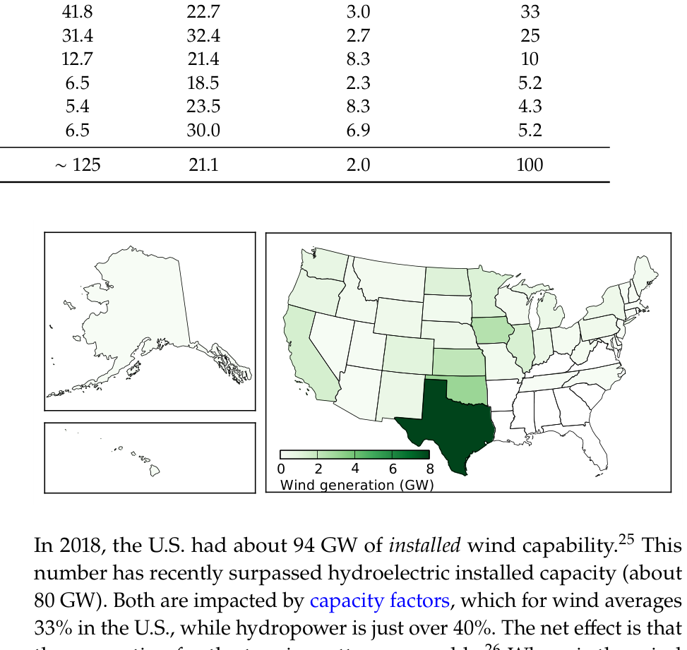
Figure 12.8:Wind power by state, in terms of average generation, in GW, in 2018. The color scale may seem unhelpful, but the unavoidable truth is that many states don’t have a lot going on, and Texas is so dominant as to render other states almost insignificant. A logarithmic color scale could help, but then the important lesson on the gross disparity might go unappreciated.
In 2018, the U.S. had about 94 GW of installed wind capability.[25] This number has recently surpassed hydroelectric installed capacity (about 80 GW). Both are impacted by capacity factors, which for wind averages 33% in the U.S., while hydropower is just over 40%. The net effect is that the generation for the two is pretty comparable.[26] Where is the wind power in the U.S. installed? Figure 12.8 shows that Texas wins, at 8.7 GW. Oklahoma is a distant second at 3.2 GW, Iowa at 2.5 GW. California is in fifth place at 1.6 GW.
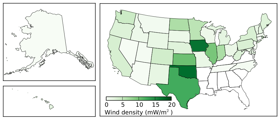
Figure 12.9:Average wind power by state, divided by state area to indicate a density of the developed resource, in milliwatts per square meter (based on 2018 data). We might expect some resemblance to Figure 12.2, based on where the resource is most favorable.
Following the flow we used in Sec. 11.3 (p. 186), we show wind generation
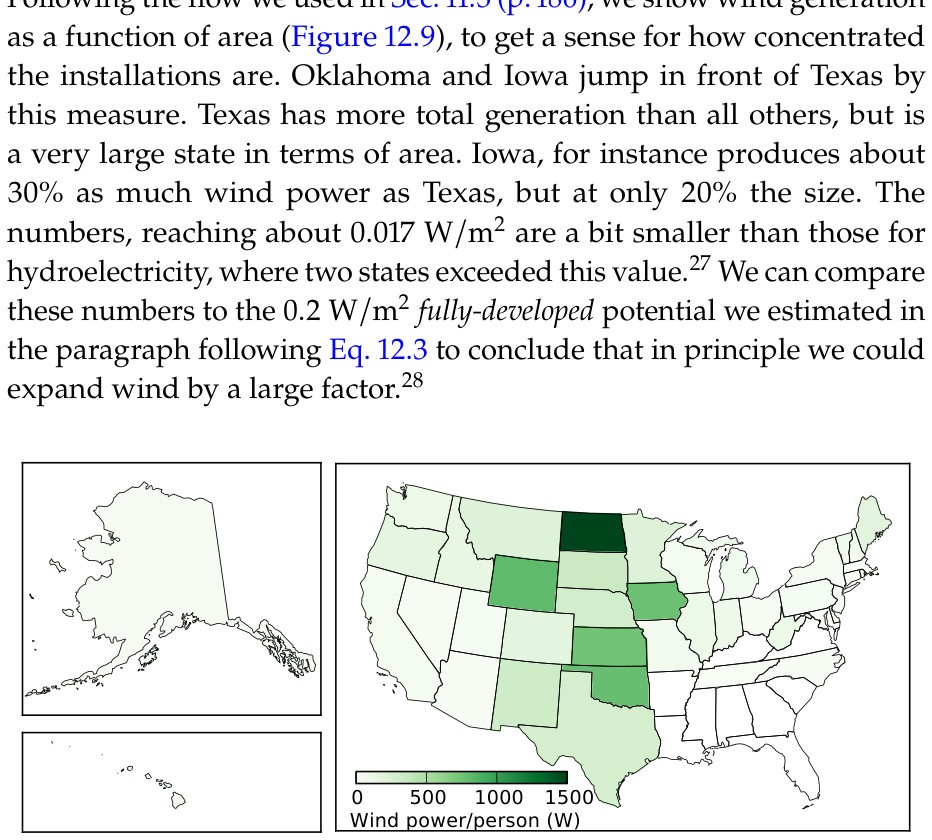
Figure 12.10:Average wind power generation by state divided by state population for an average power per person (based on 2018 data).
Next, we look at wind generation per capita in states, in Figure 12.10. Now North Dakota blows away the rest, at 1.6 kW per person, followed by four states at about half of this value. We can put this in context by noting that the average power consumption in the U.S. per capita is around 10 kW.
Finally, Figure 12.11 shows wind capacity factors, indicating where the wind is most reliable. It peaks around 41% in Kansas, but all of the plains states in general do well. The southeastern U.S. has almost no wind development,[29] as is evident in any one of these figures.
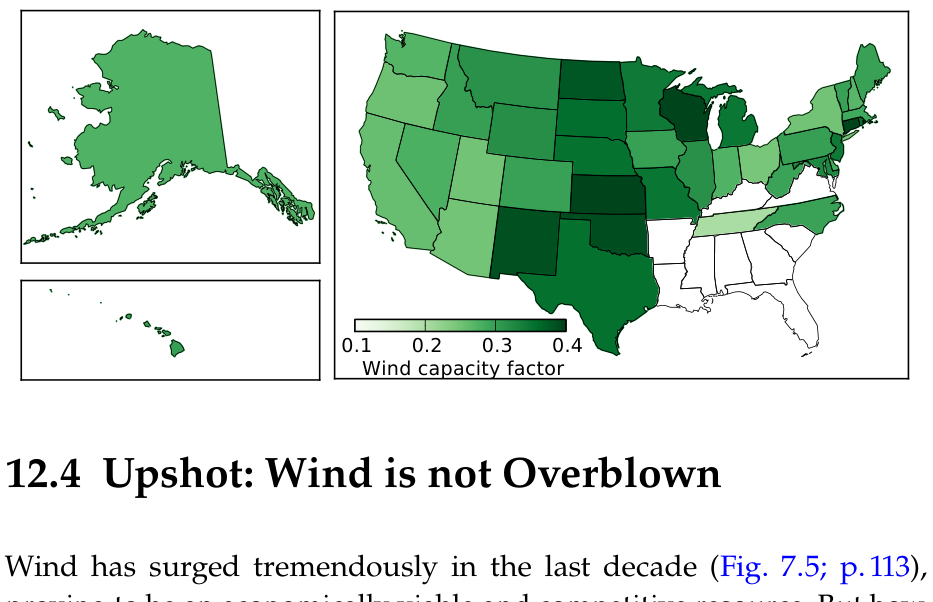
Figure 12.11:Capacity factor for wind installations by state (based on 2018 data).
12.4 Upshot: Wind is not Overblown
Wind has surged tremendously in the last decade (Fig. 7.5; p. 113), proving to be an economically viable and competitive resource. But how much could we expect to get from wind?
Putting a few of the previous results together, If the entire contiguous U.S. (area were developed for wind at an estimated power density of 0.2 —which was based on a 5 m/s average wind speed—and a capacity factor of 33%, the U.S. could theoretically produce 0.7 from wind—roughly 20 times what is produced today. We should take this crude estimate as an extreme upper end, since it is inconceivable that we would develop wind so fully as to never be more than a few hundred meters—a few rotor diameters—away from a wind turbine, no matter where we go. Also, many areas are sub-threshold and would not support investment in wind development.
Even so, the inflated 0.7 TW estimate falls short of the current 3.3 TW energy demand in the U.S., has major intermittency problems, and is not in a form that can be well-used in all sectors, like transportation and industrial processing. While wind alone cannot replace fossil fuels at the current level of demand, it can doubtless be a significant contributor.
Globally, estimates for wind potential tend to be in the few-terawatt range, though can be as low as 1 TW for a number of practical reasons [70]. As was the case for hydroelectricity, wind is a viable player in the renewables mix, but is unable to shoulder the entire load.
Wind energy is not free of environmental concerns, disturbing landscapes and habitats. Its impact on birds[31] and bats is most worrisome, as the rotors move far faster than anything to which the wildlife is habituated. Still, compared to the environmental toll from fossil fuels, it is fairly clean—similar to the impact of hydroelectric power.
A pros and cons list will help summarize. First, the positive attributes:
Wind is replenished on the planet daily by solar illumination;
Harnessing wind is relatively low-tech and straightforward;
Wind has decent efficiency—typically 40–50%—in extracting energy from the oncoming wind;
Life-cycle CO emissions for wind is only 2% that of traditional fossil fuel electricity [68];
Growth in the wind sector points to economic viability;
Wind is able to scale up to cover a meaningful fraction of energy demand.
And the downsides:
Wind is intermittent: power when nature allows, not when people demand;
Wind is regionally variable: many places do not produce enough wind to support development;
Wind can cause environmental disruption to habitats—especially dangerous to birds and bats;
Esthetic objections to noise and degradation of scenery hamper expansion.
12.5 Problems
A modest slap[32] might consist of about 1 kg of mass moving at 2 m/s. How much kinetic energy is this?
A hard slap might consist of about 1 kg of mass moving at 10 m/s. How much kinetic energy is this, and how much warmer would 10 g of skin[33] get if the skin has the heat capacity properties of water, as in the definition of a calorie (Sec. 5.5; p. 78 and Sec. 6.2; p. 90 are relevant)?
A 10 kg bowling ball falls from a height of 5 m. Using the convenient , how much gravitational potential energy does it have? Just before it hits the ground, all of this potential energy has gone into kinetic energy.[34] What is the speed of the bowling ball when it reaches the ground, based on kinetic energy?
Did the final answer for the speed of the bowling ball at the end of its drop depend on the mass?[35] Write out the math symbolically[36] and solve for velocity, . Does the result depend on mass?
Thermal energy is just randomized kinetic energy on a microscopic scale. To gain some insight into this, consider one liter (1 kg) of water, and figure out how much energy it would take to heat it from absolute zero temperature[37] to 300 K assuming that the definition of the calorie (Sec. 5.5; p. 78) applies across this entire range. If this same amount of energy went into kinetic energy—hurling the water across the room—what would the corresponding velocity be?
A typical house may have a floor area around 150 (1,600 square feet). If the floor–to-ceiling distance is typically 2.5 m, how much mass is in the air within the house? Could you lift this much mass if handed to you as bags of rocks?
Atmospheric pressure is about , meaning that a 100,000 N weight of air—corresponding to a mass of 10,000 kg—sits atop very square meter of the ground (at or near sea level). If the air density were constant at 1.25 —rather than decreasing with height as it actually does—how high would the atmosphere extend to result in this weight (mass)?
Comparing the pale green region in the southeastern U.S. to the purple region of the plains states in Figure 12.2, how much more power would we expect out of the same rotor placed in the plains than in the southeast (by what factor is it bigger in the plains)?
How much more powerful is a hurricane-strength wind of 50 m/s hitting your house than is a light breeze of 5 m/s?
How much power would a moderate-sized 50%–efficient wind turbine produce whose radius is 10 m at wind speeds of 5 m/s, 10 m/s, 15 m/s, and 20 m/s? Express the answers in kW or MW, depending on what is most natural.
The Betz limit says that we get to keep no more than 59% of the available wind power. If 59% of the kinetic energy in a lump of air moving at speed is removed, how fast is it going afterwards, as a fraction of the original speed?
The largest wind turbines have rotor diameters[40] around 150 m. Using a sensible efficiency of 50%, what power does such a jumbo turbine deliver at a maximum design wind speed of 13 m/s?
A recent news article announces the largest wind turbine yet, measuring 220 m in diameter and having a maximum power output of 13 MW. Using a reasonable efficiency, calculate the velocity of the wind at which maximum power is reached.
Compare the tip speed of a three-blade turbine operating at its optimal efficiency (as per Figure 12.4) in a moderate wind of 7 m/s to typical freeway driving speeds in the same units.
Traveling down the road, you carefully watch a three-bladed wind turbine, determining that it takes two seconds to make a full revolution. Assuming it’s operating near the peak of its efficiency curve[41] according to Figure 12.4, how fast do you infer the wind speed to be if the blade length[42] appears to be 15 m long?
Building from the result in Problem 15, how much power is this windmill delivering if its efficiency is about 50%?
In a way similar to Figure 12.5, replicate the statement in the text that the fraction of land covered per rotor area is 0.65% if turbines are separated by 15 rotor diameters along one direction and 8 rotor diameters along the cross direction.
Check that the units of Eq. 12.343 indeed are equivalent to Watts per square meter .
Provide a clear explanation of why the area under the blue curve in Figure 12.6 compared to the area of the whole rectangular box is an appropriate way to assess the capacity factor of the depicted wind farm?
What capacity factor would you estimate for the wind farm performance depicted in Figure 12.6? In other words, what is the approximate area under the curve compared to the entire box area, as explored in Problem 19? An approximate answer is fine.
Referring to Figure 12.7, examine performance at 5 m/s and at 10 m/s, picking a representative power for each in the middle of the cluster of black points, and assigning a power value from the left-hand axis. What is the ratio of power values you read off the plot, and how does this compare to theoretical expectations for the ratio going like the cube of velocity?
Figure 12.7 surprisingly has all the information required to deduce the rotor diameter! The turbine appears to produce 1,400 kW when the wind velocity is 10 m/s, and we also know it appears to operate at . What is the rotor diameter?
Considering that wind turbines are rated for the maximum-tolerable wind speed around 12 m/s, and tend to operate at about 30% capacity factor, how much average power[44] would a 100 m diameter turbine operating at 45% efficiency be expected to produce?
Table 12.2 shows Germany having more than twice the wind capability as Spain, yet each gets 8.3% of its power from wind. What do you infer the difference to be between the countries?
Do the calculation yourself to follow along.
Recall that 1 hp is 746 W. Indeed, it takes a powerful engine to provide this level of acceleration.
In this sense, “fluid” is a general term that can mean a liquid or even air.
104 kg per square meter times the surface area of Earth
In the first draft of this textbook, a different data source was used for Table 10.2 that had wind at 370 TW. Even so, the 700 TW estimate corroborated the order-of-magnitude scale and was deemed a satisfactory check: within a factor of two.
… or requiring weeks rather than a day to re-establish, once sapped
… say, within a factor of ten
We can pick any value for : a long interval makes a very long cylinder, while a small results in a short, stubby cylinder. In the end, the value we chose for will cancel out, so as not to matter.
Now it may be easier to understand why hurricanes can be so destructive, if their power scales as the cube of wind velocity, and velocities exceed 50 m/s.
Not only is the three-blade design the most efficient, its lower tip speed is less dangerous than for 2 or 1-blade designs, according to Figure 12.4.
Not too impressive: hard to get much wind power on a household scale, although 10 m/s would give 3.6 kW.
An older “rule of thumb” was 5 side-to-side and 7–8 deep, but newer work suggests as much as 8 diameters side-to-side and 15 diameters deep.
… one rotor area for every of land area
Recall that this choice gave sensible global wind power estimates lining up with Table 10.2 (p. 175).
Capacity factors for wind are smaller than for hydroelectricity due to wind being more variable than river flow.
… less than about 3 m/s; called the “cut-in” velocity
… usually around 12–15 m/s
The blades are like long airplane wings and are mounted so that they can be rotated on an axis running the length of the blade, allowing them to engage the wind at any angle, thus varying efficiency.
A typical shut-off wind speed for turbines is 20–30 m/s.
A small fraction of this is realized, due to the capacity factor.
To compare wind to total energy, we follow the thermal equivalent convention discussed for Table 10.3 (p. 177)
… as we also saw in Table 10.3 (p. 177)
Lack of wind makes it a poor fit: see also Figure 12.2.
Domestic cats turn out to kill far more birds than wind turbines do, currently.
… how painful can a few Joules be?
… corresponding to a volume of 10 mL appropriate to a slap area of 10 cm by 10 cm and to a depth of 1 mm
… neglecting any energy flow to air resistance
Try it using a different mass.
… using variables/symbols
… 0 K, when the kinetic energy is effectively frozen out, or stopped
⚠ not radius
Hint: focus on tip speed.
… corresponding to radius of the rotor
Hint: compute power at 12 m/s then apply capacity factor