Skip to article frontmatterSkip to article content
Site not loading correctly?

This may be due to an incorrect BASE_URL configuration. See the MyST Documentation for reference.

10. Oscillatory Motion

King Abdullah University of Science and Technology

10.1 Oscillatory Motion

A motion repeating itself is referred to as periodic or oscillatory motion. An object in such motion oscillates about an equilibrium position due to a restoring force or torque. Such force or torque tends to restore (return) the system toward its equilibrium position no matter in which direction the system is displaced. This motion is important to study many phenomena including electromagnetic waves, alternating current circuits, and molecules. For a vibration to occur, two quantities are necessary to be present—stiffness and inertia.

10.2 Free Vibrations

When a system vibrates, a restoring force must be present. In addition to that force, there is always a retarding or damping force such as friction. If the effect of the damping force is small and can be neglected, then the motion is classified as free and undamped motion. Otherwise, the motion is classified as free damped motion. In both cases, the motion is known as free vibration since no forces other than the restoring and damping forces exist during vibration. If a driving force that does positive work on the system exists, the motion is classified as forced vibration.

This force may be applied externally to the system or sometimes is produced within the system. In this chapter, the case in which a restoring force is directly proportional to the displacement is considered. The resulting motion is then known as a harmonic vibration and the system is said to be linear. If the restoring force depends on the displacement in some other way, the resulting motion is known as anharmonic vibration and the system is said to be nonlinear.

10.3 Free Undamped Vibrations

This kind of motion is known as the simple harmonic motion. Next, we will examine examples of such motion in physics.

10.3.1 Mass Attached to a Spring

Consider a block of mass m attached to a light spring of spring constant k that is fixed at the other end (see Figure 1). Suppose that the system lies on a frictionless horizontal surface. For small displacements, the restoring force acting on the block by the spring is given by Hook’s law

Fs=kxF_{s}=-kx

As we’ve mentioned in 4.1 Introduction, if the block is displaced slightly to the right (for example to x=Ax=A), the restoring spring force will accelerate the block to the left transferring its potential energy into kinetic energy As the block reaches its equilibrium position x=0x=0, all of its potential energy will be transformed into kinetic energy and it will overshoot to the other side. Again, as it moves left, the spring force decelerates the block to the right, transferring its kinetic energy into potential energy until all of its energy is potential at x=Ax= -A where it comes to rest. At that point, it accelerates back to x=0x=0 and regains all of its kinetic energy where it overshoots again to x=Ax=A. Therefore, stiffness restores the mass where inertia is responsible for the mass to overshoot. From Newton’s second law we, have

ma=kxma=-kx

or

md2xdt2+kx=0m\frac{d^{2}x}{dt^{2}}+kx=0

or

d2xdt2+ωn2x=0\begin{aligned} \frac{d^{2}x}{dt^{2}}+\omega _{n}^{2}x=0 \end{aligned}

where ωn=k/m\omega _{n}=\sqrt{k/m} is called the natural angular frequency of the system. The general solution of this equation is of the form

x(t)=A1cosωnt+A2sinωnt\begin{aligned} x(t)=A_{1}\cos \omega _{n}t+A_{2}\sin \omega _{n}t \end{aligned}

where A1A_{1} and A2A_{2} are arbitrary constants that can be found from the initial conditions. Therefore, there are many possible motions with the same angular frequency ωn\omega _{n}. By multiplying and dividing (5) by A12+A22\sqrt{A_{1}^{2}+A_{2}^{2}}, you can show that the solution may be written as

x(t)=Acos(ωntϕ)\begin{aligned} x(t)=A\cos (\omega _{n}t-\phi ) \end{aligned}

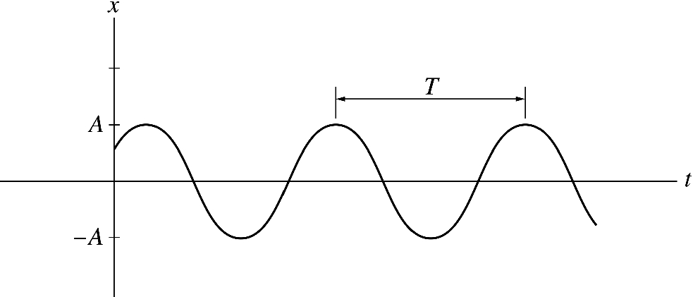
where A=A12+A22A=\sqrt{A_{1}^{2}+A_{2}^{2}} is called the amplitude of motion and ϕ=tan1A2/A1\phi =\tan ^{-1}A_{2}/A_{1} is called the phase constant. In general, ϕ\phi is chosen such that 0ϕπ.A0\le \phi \le \pi. A and ϕ\phi can be determined from the initial conditions, i.e., from the values of the displacement and velocity when the motion starts. The mass therefore oscillates between A and A-A. The quantity (ωntϕ)(\omega _{n}t-\phi ) is called the phase angle. If this angle is increased by 2π2\pi, all physical quantities such as the displacement, velocity, and acceleration repeat themselves. The plot of x versus t is shown in Figure 2. If A is fixed and ϕ\phi is changed the motion will be the same except that the same physical quantities will appear either earlier or later than the preceding motion.

A block of mass m attached to a light spring of spring constant k that is fixed at the other end

Figure 1:A block of mass m attached to a light spring of spring constant k that is fixed at the other end

Plot of x versus t for a simple harmonic oscillator

Figure 2:Plot of x versus t for a simple harmonic oscillator

10.3.1.1 The Period and Frequency of Motion

The period of motion is the time required for one complete cycle or oscillation. Since the phase angle is changed by 2π2\pi after one complete cycle, we have for the mass–spring system,

ωnt+2π=ωn(t+T)\omega _{n}t+2\pi =\omega _{n}(t+T)

or

T=2πωn=2πmkT=\frac{2\pi }{\omega _{n}}=2\pi \sqrt{\frac{m}{k}}

The frequency is defined as the number of complete cycles per unit time

fn=1T=ωn2πf_{n}=\frac{1}{T}=\frac{\omega _{n}}{2\pi }

This frequency is called the natural frequency of the motion. The unit of the frequency is cycles/s or hertz (Hz).

10.3.1.2 The Phase Difference

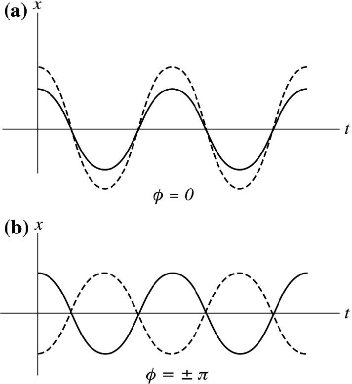
The phase constant ϕ\phi is important when comparing two or more oscillations of the same frequency Suppose a certain vibration has ϕ=0\phi =0, this means that at t=0t=0 the displacement is maximum x=Ax=A. If a second vibration has also ϕ=0\phi =0, then the two vibrations are said to be in phase (see Figure 3 part a). Otherwise, the two vibrations are out of phase. If the phase constant of the second vibration is ϕ>0\phi >0, then the second vibration is leading the first vibration in phase by ϕ\phi. If ϕ<0\phi <0, then the second vibration is lagging the first by ϕ\phi. If ϕ=±π\phi =\pm \pi, the two vibrations are said to be in antiphase with each other (see Figure 3 part b).

a Two simple harmonic motions of the same frequency and same phase constant \pi =0 but differing in amplitude. b Two simple harmonic motions of the same frequency and amplitude but differing in phase by \phi =\pm \pi

Figure 3:a Two simple harmonic motions of the same frequency and same phase constant π=0\pi =0 but differing in amplitude. b Two simple harmonic motions of the same frequency and amplitude but differing in phase by ϕ=±π\phi =\pm \pi

10.3.1.3 The Velocity and Acceleration

The velocity of the mass is

v(t)=dxdt=ωnAsin(ωntϕ)\begin{aligned} v(t)=\frac{dx}{dt}=-\omega _{n}A\sin (\omega _{n}t-\phi ) \end{aligned}

This can also be written as

v(t)=ωnAcos(ωntϕ+π2)\begin{aligned} v(t)=\omega _{n}A\cos \bigg (\omega _{n}t-\phi +\frac{\pi }{2}\bigg ) \end{aligned}

The acceleration of the mass is

a(t)=dvdt=ωn2Acos(ωntϕ)\begin{aligned} a(t)=\frac{dv}{dt}=-\omega _{n}^{2}A\cos (\omega _{n}t-\phi ) \end{aligned}

or

a(t)=dvdt=ωn2Acos(ωntϕ+π)\begin{aligned} a(t)=\frac{dv}{dt}=\omega _{n}^{2}A\cos (\omega _{n}t-\phi +\pi ) \end{aligned}

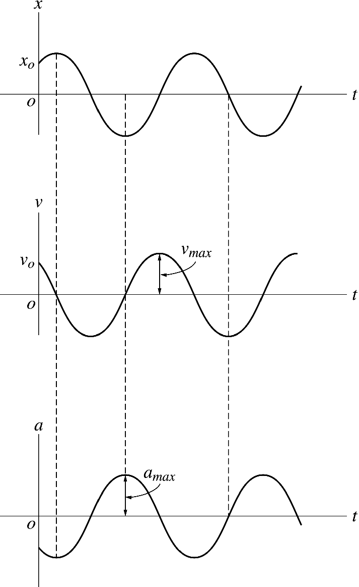
Hence, the velocity and acceleration also vary harmonically with time with amplitudes ωnA\omega _{n}A and ωn2A\omega _{n}^{2}A, respectively, but they all have the same angular frequency From Eqs. 10.5 and 10.7 you can see that the velocity leads the displacement by π/2\pi /2 or 90. The acceleration on the other hand leads the velocity by π/2\pi /2 and the displacement by π\pi or 180. Figure 10.4 shows the displacement, velocity, and acceleration versus time.

The displacement, velocity and acceleration versus time

Figure 4:The displacement, velocity and acceleration versus time

10.3.1.4 Boundary Conditions

Boundary conditions are used to find A and ϕ\phi for a specific vibration. Suppose that the vibration is measured when the stopwatch is set to zero, i.e., at t=0t=0 and that at that instant the mass is released from rest at a distance of x=A1x=A_{1} from its equilibrium position. Substituting these conditions into Eqs. 10.3 and 10.4, we have

x=Acosϕ=A1\begin{aligned} x=A\cos \phi =A_{1} \end{aligned}
v=v0=ωnAsinϕ\begin{aligned} v=v_{0}=-\omega _{n}A\sin \phi \end{aligned}

Dividing (15) by (14) gives

tanϕ=v0ωnA1\tan \phi =\frac{-v_{0}}{\omega _{n}A_{1}}

Squaring and adding Eqs. 10.9 and 10.8 gives

A12+(v0ωn)2=A2cos2ϕ+A2sin2ϕA_{1}^{2}+\bigg (\frac{v_{0}}{\omega _{n}}\bigg )^{2}=A^{2}\cos ^{2}\phi +A^{2}\sin ^{2}\phi

or

A=A12+(v0ωn)2A=\sqrt{A_{1}^{2}+\bigg (\frac{v_{0}}{\omega _{n}}\bigg )^{2}}
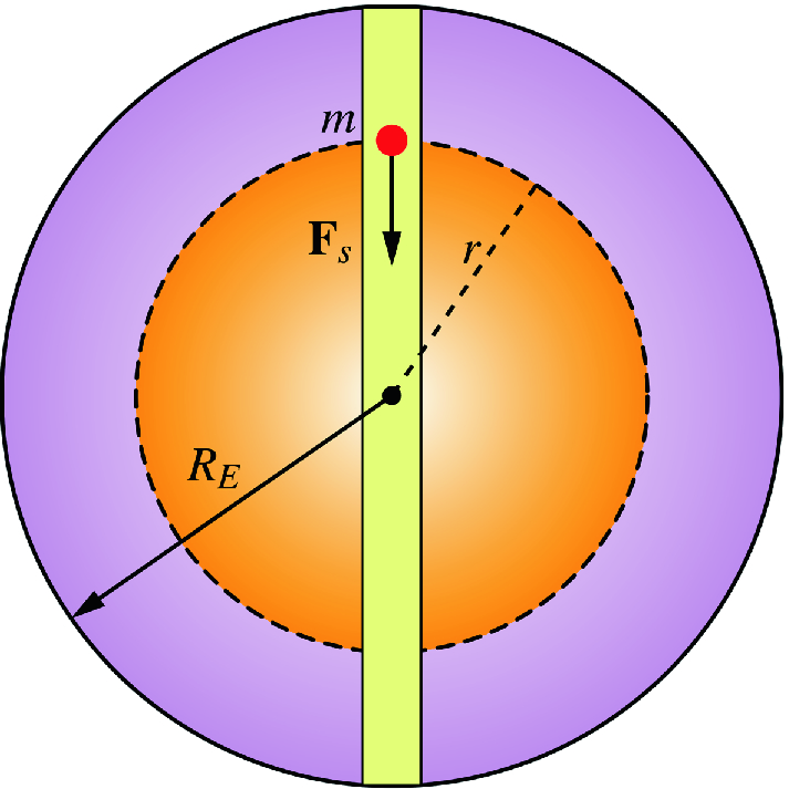
A particle of mass m is dropped in a straight tunnel that is drilled through the earth and which passes through the center of earth

Figure 5:A particle of mass m is dropped in a straight tunnel that is drilled through the earth and which passes through the center of earth

A block connected to two springs

Figure 6:A block connected to two springs

A second block on top of a block connected to a spring

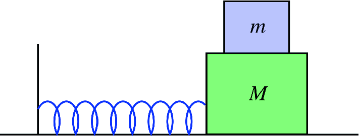
Figure 7:A second block on top of a block connected to a spring

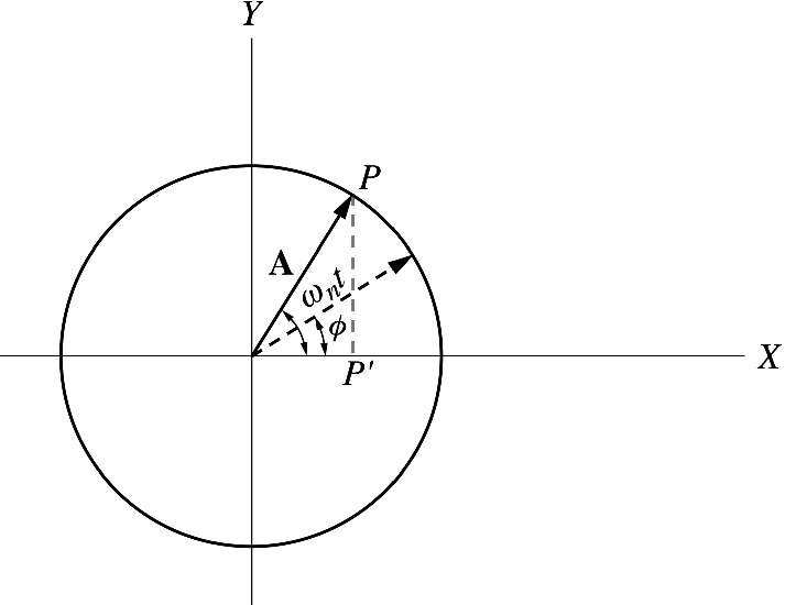
A particle in uniform circular motion

Figure 8:A particle in uniform circular motion

10.3.2 Simple Harmonic Motion and Uniform Circular Motion

Consider a circle of radius A centered at the x\mathrm {x} and y\mathrm {y} axes as shown in Figure 8. Let A be the position vector of a particle P\mathrm {P} rotating with a constant angular speed ωn\omega _{n} in the anticlockwise direction. The particle is thus in uniform circular motion. Suppose P\mathrm {P} starts the rotation at t=0t=0 at an angle of ϕ\phi measured from the positive x\mathrm {x}-axis. At any time, the angular position of the particle is given by (ωnt+ϕ)(\omega _{n}t+\phi ), therefore the vector position of the particle at any time is

A=xi+yj=Acos(ωnt+ϕ)i+Asin(ωnt+ϕ)j\mathbf {A}=x\mathbf {i}+y\mathbf {j}=A\cos (\omega _{n}t+\phi )\mathbf {i}+A\sin (\omega _{n}t+\phi )\mathbf {j}

Hence,

x=Acos(ωnt+ϕ)x=A\cos (\omega _{n}t+\phi )

and

y=Asin(ωnt+ϕ)y=A\sin (\omega _{n}t+\phi )

That is, as P\mathrm {P} moves in uniform circular motion, its projection P\mathrm {P}' on the x-axis moves in simple harmonic motion where the radius of the circle is equal to the amplitude of motion. The projection of P\mathrm {P} along the y\mathrm {y}-axis also undergoes simple harmonic motion. Thus, uniform circular motion may be considered as a combination of the simple harmonic motions of the projections of P\mathrm {P} on each axis. These two simple harmonic motions have equal amplitudes and angular frequencies but are in quadrature with each other (they differ in phase by π/2\pi /2). The linear tangential velocity of the particle in this uniform circular motion is given by

v=Aωnv=A\omega _{n}

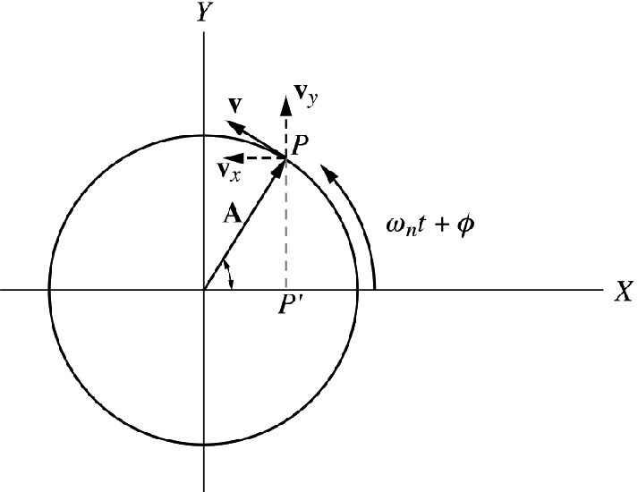
The x\mathrm {x} component of the velocity is from Figure 9 given by

vx=ωnAsin(ωnt+ϕ)v_{x}=-\omega _{n}A\sin (\omega _{n}t+\phi )

The acceleration of the particle in uniform circular motion is just the radial (centripetal) acceleration that is given by

a=v2A=Aωn2a=\frac{v^{2}}{A}=A\omega _{n}^{2}

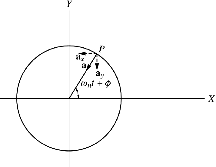
The x\mathrm {x} components of the acceleration (see Figure 10) is

ax=ωn2Acos(ωnt+ϕ)a_{x}=-\omega _{n}^{2}A\cos (\omega _{n}t+\phi )

Hence as you can see, the displacement, velocity, and acceleration of the projection of P\mathrm {P} onto the x\mathrm {x} (or y\mathrm {y} axis) are the same as that of a simple harmonic motion. From this, we conclude that the simple harmonic motion can be represented as the projection of uniform circular motion along a diameter of the circle.

The velocity components of the particle

Figure 9:The velocity components of the particle

The acceleration components of the particle

Figure 10:The acceleration components of the particle

10.3.3 Energy of a Simple Harmonic Oscillator

Since in a simple harmonic oscillator, there aren’t any dissipative forces, the total mechanical energy of the system is conserved and is equal to the sum of its kinetic and potential energies, that is

E=K+UE=K+U
K=12mv2=12mωn2A2sin2(ωnt+ϕ)K=\frac{1}{2}mv^{2}=\frac{1}{2}m\omega _{n}^{2}A^{2}\sin ^{2}(\omega _{n}t+\phi )
U=12kx2=12kA2cos2(ωnt+ϕ)U=\frac{1}{2}kx^{2}=\frac{1}{2}kA^{2}\cos ^{2}(\omega _{n}t+\phi )

Thus,

E=12kA2[sin2(ωnt+ϕ)+cos2(ωnt+ϕ)]E=\frac{1}{2}kA^{2}[\sin ^{2}(\omega _{n}t+\phi )+\cos ^{2}(\omega _{n}t+\phi )]

or

E=12kA2=constantE=\frac{1}{2}kA^{2}= \text {constant}

The equation of motion of a simple harmonic oscillator can be obtained from the total mechanical energy of the system as follows:

E=12mx˙2+12kx2=12kA2\begin{aligned} E=\frac{1}{2}m\dot{x}^{2}+\frac{1}{2}kx^{2}=\frac{1}{2}kA^{2} \end{aligned}
dEdt=mx˙x¨+kxx˙=0\frac{dE}{dt}=m\dot{x}\ddot{x}+kx\dot{x}=0

or

mx¨+kx=0m\ddot{x}+kx=0

Hence

x¨+ωn2x=0\ddot{x}+\omega _{n}^{2}x=0

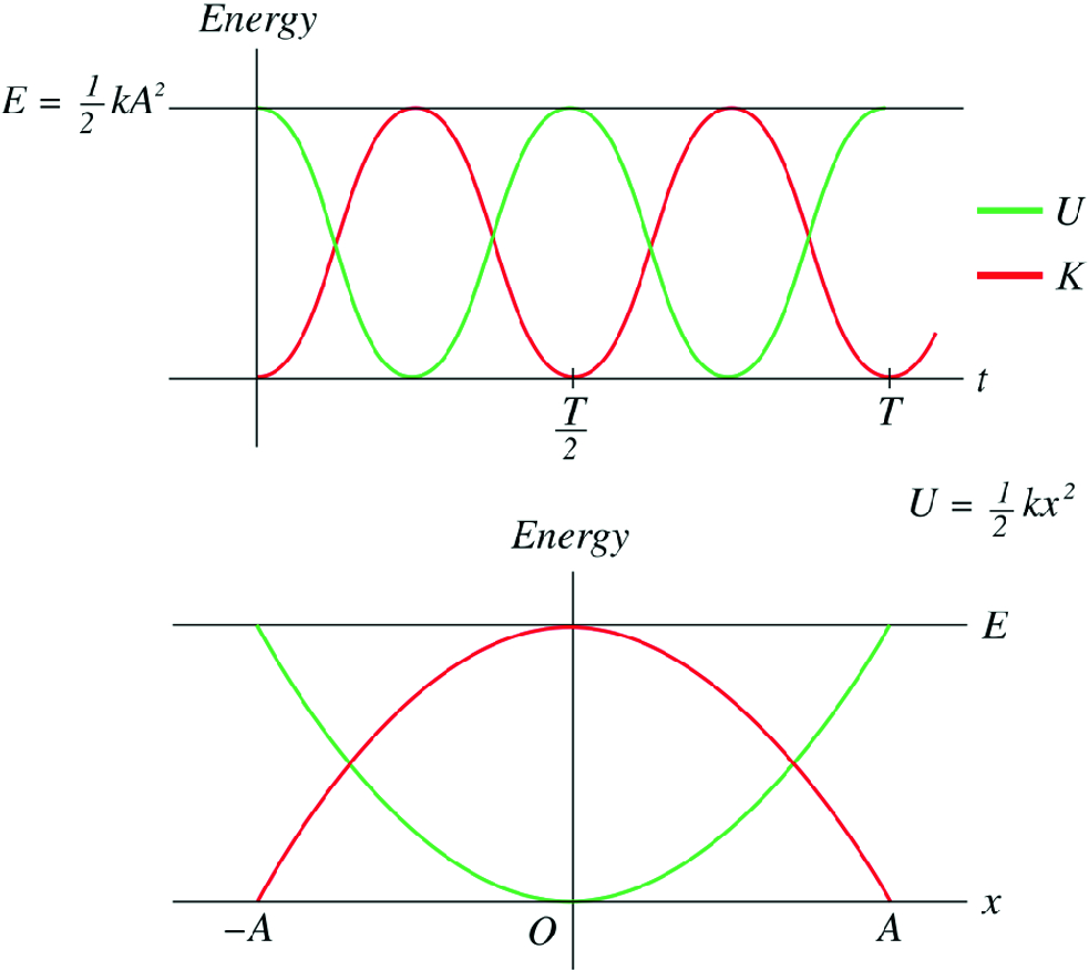
where ωn=k/m\omega _{n}=\sqrt{k/m}. As the mass moves, its kinetic energy is transformed into potential energy and vice versa. Figure 10.11 shows the kinetic energy and potential energy of the system as a function of time and as a function of the displacement respectively Note that the variation of U and K with time is at twice the angular frequency of the variation of x, v, and a with time. This is because the potential energy is converted to kinetic energy twice in each cycle. The velocity of the simple harmonic oscillator can be obtained from the total energy of the system. From (60), we have

v=±km(A2x2)v=\pm \sqrt{\frac{k}{m}(A^{2}-x^{2})}

Hence, the maximum speed is at x=0x=0 and is zero at x=±Ax=\pm A which are called the turning points as discussed in Chap. chap444.

As the mass moves, its kinetic energy is transformed into potential energy and vice versa

Figure 11:As the mass moves, its kinetic energy is transformed into potential energy and vice versa

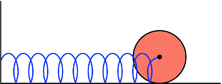
A solid cylinder connected to a light spring

Figure 12:A solid cylinder connected to a light spring

10.3.4 The Simple Pendulum

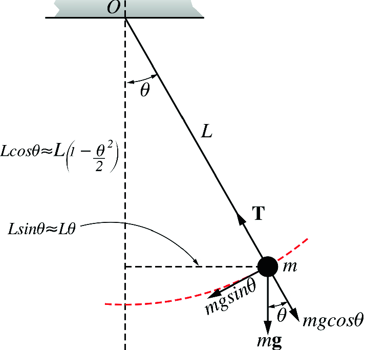
The simple pendulum is an example of an angular vibration in which the restoring effect is due to a restoring torque. A simple pendulum consists of a mass (called the bob) suspended by a light string of length L that is fixed at the other end (see Figure 13). If the mass is pulled to the right or left from its equilibrium position and released, then the pendulum will swing in a vertical plane about an axis passing through O. The resulting motion is then a periodic or oscillatory motion. The restoring torque is due to gravity and is given by

τ=(mgsinθ)L\tau =-(mg\sin \theta )L

The minus sign indicates that the torque is a restoring torque, since it always tends to decrease θ\theta. The moment of inertia of the bob about an axis passing through O\mathrm {O} is

I=mL2I=mL^{2}

From Newton’s second law in angular form, we have

τ=Iα=Iθ¨\tau =I\alpha =I\ddot{\theta }

Hence,

mgsinθL=mL2θ¨-mg\sin \theta L=mL^{2}\ddot{\theta }

or

θ¨+(gL)sinθ=0\begin{aligned} \ddot{\theta }+\bigg (\frac{g}{L}\bigg )\sin \theta =0 \end{aligned}

This equation does not represent a harmonic motion. That is because the torque is not directly proportional to the angular displacement. Thus, the system is nonlinear. However for small angular displacements, we have sinθθ(\sin \theta \approx \theta (since sinθ=θθ3/3!+θ5/5!)\sin \theta =\theta -\theta ^{3}/3!+\theta ^{5}/5!\ldots ) and (93) becomes

θ¨+(gL)θ=0\ddot{\theta }+\bigg (\frac{g}{L}\bigg )\theta =0

or

θ¨+ωn2θ=0\begin{aligned} \ddot{\theta }+\omega _{n}^{2}\theta =0 \end{aligned}

where ωn=g/L\omega _{n}=\sqrt{g/L}. Hence for small angular displacements, the motion is a simple harmonic motion. The solution of (95) is of the form

θ=θmcos(ωntϕ)\theta =\theta _{m}\cos (\omega _{n}t-\phi )

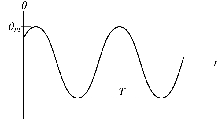
where θm\theta _{m} is the maximum angular displacement and ϕ\phi is the phase constant. The plot of this equation is shown in Figure 14. The period of the simple pendulum is therefore given by

T=2πωn=2πLgT=\frac{2\pi }{\omega _{n}}=2\pi \sqrt{\frac{L}{g}}
The simple pendulum

Figure 13:The simple pendulum

The displacement versus time of a simple pendulum

Figure 14:The displacement versus time of a simple pendulum

10.3.4.1 Energy

The kinetic energy of the simple pendulum is

K=12mv2=12mL2ωn2=12mLθ˙2K=\frac{1}{2}mv^{2}=\frac{1}{2}mL^{2}\omega _{n}^{2}=\frac{1}{2}mL\dot{\theta }^{2}

Taking the reference point of potential energy of the system to be zero when the bob is at the bottom, we have

U=MgL(1cosθ)U=MgL(1-\cos \theta )

The total energy is therefore given by

E=K+U=12ML2θ˙2+MgL(1cosθ)E=K+U=\frac{1}{2}ML^{2}\dot{\theta }^{2}+MgL(1-\cos \theta )

For small θ\theta, we have cosθ1θ22\cos \theta \approx 1-\frac{\theta ^{2}}{2}since cosθ=1θ2/2!+θ4/4!)\cos \theta =1-\theta ^{2}/2!+\theta ^{4}/4!\ldots ) thus

E=12ML2θ˙2+12MgLθ2E=\frac{1}{2}ML^{2}\dot{\theta }^{2}+\frac{1}{2}MgL\theta ^{2}

Since

θ˙=θmωnsin(ωntϕ)\dot{\theta }=-\theta _{m}\omega _{n}\sin (\omega _{n}t-\phi )

we have

E=12ML2θm2ωn2sin2(ωntϕ)+12MgLθm2cos2(ωntϕ)E=\frac{1}{2}ML^{2}\theta _{m}^{2}\omega _{n}^{2}\sin ^{2}(\omega _{n}t-\phi )+\frac{1}{2}MgL\theta _{m}^{2}\cos ^{2}(\omega _{n}t-\phi )

or

E=12MgLθm2E=\frac{1}{2}MgL\theta _{m}^{2}

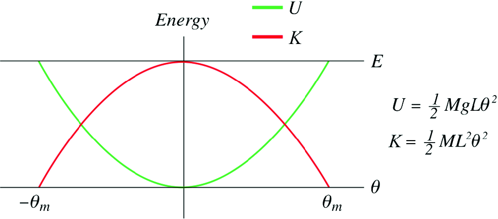
Therefore, the total energy of the system is constant. Figure 10.15 shows the variation of the kinetic and potential energies with the displacement.

The total energy of a simple pendulum

Figure 15:The total energy of a simple pendulum

The equation of motion may also be obtained from energy as follows:

dEdt=ML2θ˙θ¨+MgLθθ˙=0\frac{dE}{dt}=ML^{2}\dot{\theta }\ddot{\theta }+MgL\theta \dot{\theta }=0

or

θ¨+(gL)θ=0\ddot{\theta }+\bigg (\frac{g}{L}\bigg )\theta =0
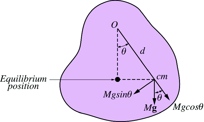
The physical pendulum

Figure 16:The physical pendulum

10.3.5 The Physical Pendulum

The physical pendulum is a rigid body that oscillates about an axis passing through a point in the body other than its center of mass (the center of mass is assumed to be located at the center of gravity). Figure 10.16 shows a rigid body pivoted at point O\mathrm {O} that is at a distance d from the center of mass. The equilibrium position of the body is when its center of mass is directly below the pivot O. If the body is displaced either to the right or left from the equilibrium position, a restoring torque due to gravity will act on it. As a result, the body will oscillate in a vertical plane where the axis of rotation is perpendicular to the page. The restoring torque is given by

τ=Mgd sinθ\tau =-Mgd\ \sin \theta

where M is the mass of the body and d is the moment arm of the tangential component of the weight (Mg sinθ)(Mg\ \sin \theta ). From Newton’s second law, we have

τ=Iα\tau =I\alpha
Mgdsinθ=Iθ¨-Mgd\sin \theta =I\ddot{\theta }

For small angular displacements sinθθ\sin \theta \approx \theta and hence

θ¨+(MgdI)θ=0\ddot{\theta }+\bigg (\frac{Mgd}{I}\bigg )\theta =0

or

θ¨+ωn2θ=0\ddot{\theta }+\omega _{n}^{2}\theta =0

This equation is of a simple harmonic motion with an angular frequency of

ωn=MgdI\omega _{n}=\sqrt{\frac{Mgd}{I}}

and a period of motion of

T=2πωn=2πIMgdT=\frac{2\pi }{\omega _{n}}=2\pi \sqrt{\frac{I}{Mgd}}

Thus,

I=T2Mgd4π2I=\frac{T^{2}Mgd}{4\pi ^{2}}

Therefore, the moment of inertia of a body can be found by measuring its period when it is in simple harmonic motion as a physical pendulum. Note that, the simple pendulum is a special case of the physical pendulum since for a simple pendulum of mass m, the moment of inertia is

I=md2I=md^{2}

and thus, the angular frequency is

ωn=mgdmd2=gd\omega _{n}=\sqrt{\frac{mgd}{md^{2}}}=\sqrt{\frac{g}{d}}

This angular frequency is of a simple pendulum where d represents the length of the string.

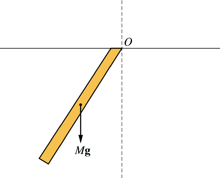
A uniform rod suspended at one end oscillated with a small amplitude

Figure 17:A uniform rod suspended at one end oscillated with a small amplitude

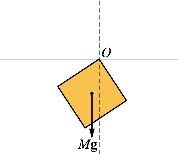
A uniform square plate pivoted at one of its corners and oscillates in a vertical plane

Figure 18:A uniform square plate pivoted at one of its corners and oscillates in a vertical plane

The torsional pendulum

Figure 19:The torsional pendulum

10.3.6 The Torsional Pendulum

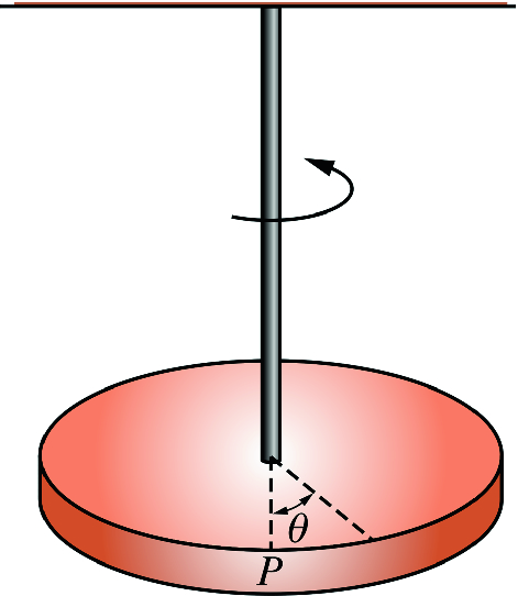
The torsional pendulum consists of a rigid body suspended by a wire from its center of mass where the other end of the wire is fixed as shown in Figure 19. The body is in equilibrium if the wire is untwisted. If the body is rotated through an angle θ\theta it will oscillate about its equilibrium position (the line OP) due to a restoring torque exerted by the twisted wire on the body. This torque is found to be directly proportional to the angular displacement of the body. That is

τ=kθ\tau =-k\theta

where k is called the torsional constant. Its value depends on the property of the wire. Note that this equation is the rotational analogue of Hook’s law in linear form (F=kx)(F=-kx). From Newton’s second law, we have

τ=Iα\tau =I\alpha

or

kθ=Iθ¨-k\theta =I\ddot{\theta }

That gives

θ¨+(kI)θ=0\ddot{\theta }+\bigg (\frac{k}{I}\bigg )\theta =0

or

θ¨+ωn2θ=0\ddot{\theta }+\omega _{n}^{2}\theta =0

where ωn=k/I\omega _{n}=\sqrt{k/I} and the period is T=2πI/k.T=2\pi \sqrt{I/k}.

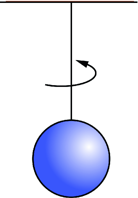
A uniform solid sphere suspended at its midpoint by a light string

Figure 20:A uniform solid sphere suspended at its midpoint by a light string

10.4 Damped Free Vibrations

In this section, we will discuss the case in which the effect of damping that is due to a nonconservative force cannot be neglected. An example of such a force in mechanical systems is the force of friction. In this case, the mechanical energy of the system will be lost, the amplitude of motion will decrease to zero, and the oscillation dies out eventually. Here, we will discuss damping due to friction in the simplest case, where the frictional force is proportional to the first power of the velocity of the oscillating body. An example of such a frictional force is the force that an object experience when moving in a fluid with a low speed and is given by

FD=bvF_{D}=-bv

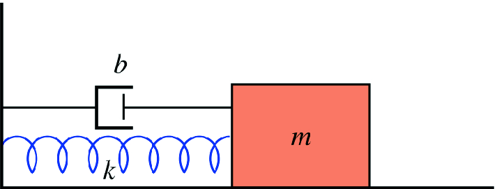
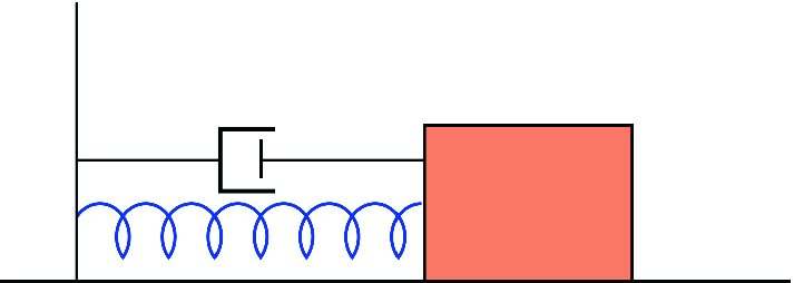
where b is a positive constant called the damping coefficient. Its SI units is N(ms1)=kgs1\mathrm {N}(\mathrm {m}\,\mathrm {s}^{-1})=\mathrm {k}\mathrm {g}\,\mathrm {s}^{-1}. The negative sign shows that the direction of the force is always opposite to the velocity. Now consider the spring–mass system as shown in Figure 21, the cylinder shown in the figure contains a viscous fluid and a piston moving in it. Such device is known as the viscous damper. The net force on the oscillating body is

A mass-spring system with damping

Figure 21:A mass-spring system with damping

F=Fs+FD=kxbv\sum F=F_{s}+F_{D}=-kx-bv

hence

mx¨+bx˙+kx=0m\ddot{x}+b\dot{x}+kx=0

or

x¨+γx˙+ωn2x=0\begin{aligned} \ddot{x}+\gamma \dot{x}+\omega _{n}^{2}x=0 \end{aligned}

where γ=b/m\gamma =b/m and ωn=k/m\omega _{n}=\sqrt{k/m}. The units of γ\gamma is s1\mathrm {s}^{-1}. This equation is a second order linear differential equation of constant coefficients. We may assume a solution of the form

x=Ceλtx=Ce^{\lambda t}

Substituting this solution into (144) gives the characteristic (auxiliary) equation given by

λ2+γλ+ωn2=0\lambda ^{2}+\gamma \lambda +\omega _{n}^{2}=0

The roots of this equation are given by

λ1=γ2+(γ24ωn2)\lambda _{1}=-\frac{\gamma }{2}+\sqrt{\bigg (\frac{\gamma ^{2}}{4}-\omega _{n}^{2}\bigg )}

and

λ2=γ2(γ24ωn2)\lambda _{2}=-\frac{\gamma }{2}-\sqrt{\bigg (\frac{\gamma ^{2}}{4}-\omega _{n}^{2}\bigg )}

From superposition, the general solution is given by

x=C1eλ1t+C2eλ2t\begin{aligned} x=C_{1}e^{\lambda _{1}t}+C_{2}e^{\lambda _{2}t} \end{aligned}

Three possible solutions arise depending on whether the sign of the bracket (γ2/4ωn2)(\gamma ^{2}/4-\omega _{n}^{2}) is positive, negative or zero, i.e., depending on the size of the damping force. The roots λ1\lambda _{1} and λ2\lambda _{2} are either distinct real roots, equal real roots or a conjugate complex roots. Therefore, there are three possible motions of the system.

10.4.1 Light Damping (Under-Damped) (γ<2ωn)(\gamma <2\omega _{n})

If γ<2ωn\gamma <2\omega _{n} the resulting roots are complex roots given by

λ1=γ2+iωD\lambda _{1}=-\frac{\gamma }{2}+i\omega _{D}

and

λ2=γ2iωD\lambda _{2}=-\frac{\gamma }{2}-i\omega _{D}

where

ωD=(ωn2γ24)1/2\omega _{D}=\bigg (\omega _{n}^{2}-\frac{\gamma ^{2}}{4}\bigg )^{1_{/2}}

Hence, (149) may be written as

x=[C1eiωDt+C2eiωDt]eγ2tx=\bigg [C_{1}e^{i\omega _{D}t}+C_{2}e^{-i\omega _{D}t}\bigg ]e^{\frac{-\gamma }{2}t}

Since e±ix=cosx±isinxe^{\pm ix}=\cos x\pm i\sin x we have

x=[C1(cosωDt+isinωDt)+C2(cosωDtisinωDt)]eγ2tx=[C_{1}(\cos \omega _{D}t+i\sin \omega _{D}t)+C_{2}(\cos \omega _{D}t-i\sin \omega _{D}t)]e^{\frac{-\gamma }{2}t}
=[(C1+C2)cosωDt+i(C1C2)sinωDt]eγ2t=[(C_{1}+C_{2})\cos \omega _{D}t+i(C_{1}-C_{2})\sin \omega _{D}t]e^{\frac{-\gamma }{2}t}
=[A1cosωDt+A2sinωDt]eγ2t\begin{aligned} =[A_{1}\cos \omega _{D}t+A_{2}\sin \omega _{D}t]e^{\frac{-\gamma }{2}t} \end{aligned}

where A1=C1+C2A_{1}=C_{1}+C_{2} and A2=i(C1C2)A_{2}=i(C_{1}-C_{2}). As mentioned earlier (156) can be written as

x=Acos(ωDtϕ)eγ2t\begin{aligned} x=A\cos (\omega _{D}t-\phi )e^{\frac{-\gamma }{2}t} \end{aligned}

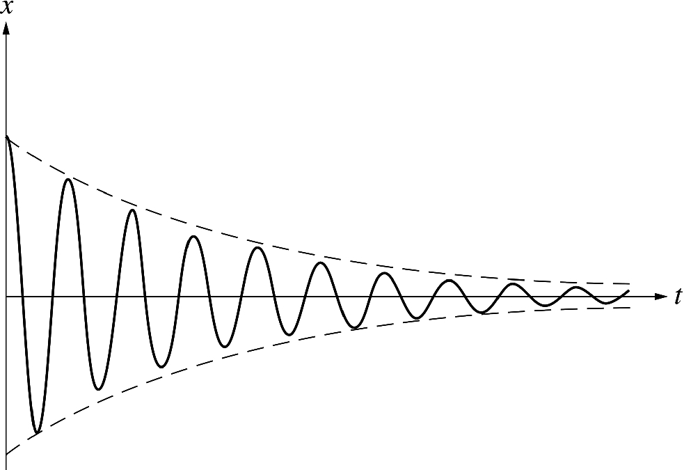
where A is the initial amplitude of motion. Aeγ2tAe^{\frac{-\gamma }{2}t} is called the amplitude of motion and ϕ\phi is the phase constant and ωD\omega _{D} is the angular frequency of the damped motion. This equation shows that the system oscillates in a decreasing harmonic motion where the amplitude of motion decreases exponentially with time until eventually the oscillation dies out (see Figure 22). The dashed lines in Figure 22 are called the envelope of the oscillation curve. The period of motion in light damping is therefore given by

τD=2πωD=2πωn2γ24\tau _{D}=\frac{2\pi }{\omega _{D}}=\frac{2\pi }{\sqrt{\omega _{n}^{2}-\frac{\gamma ^{2}}{4}}}

If b=0b=0 and thus γ=0\gamma =0 the period of motion is reduced to that of a simple harmonic oscillator. If γωD\gamma \ll \omega _{D}, the situation is referred to as very light damping and ωDωn\omega _{D}\approx \omega _{n}. Furthermore if there are two amplitudes AaA_{a} and AbA_{b} separated by the period of motion, then their ratio is given by

AaAb=Aeγ2t1Aeγ2(t1+τD)=eγ2τD\frac{A_{a}}{A_{b}}=\frac{Ae^{-\frac{\gamma }{2}t_{1}}}{Ae^{-\frac{\gamma }{2}(t_{1}+\tau _{D})}}=e^{\frac{\gamma }{2}\tau _{D}}

A quantity known as the logarithmic decrement is defined as

δ=ln(AaAb)=γ2τD\delta =\ln \bigg (\frac{A_{a}}{A_{b}}\bigg )=\frac{\gamma }{2}\tau _{D}
In A lightly damped oscillator, the system oscillates in a decreasing harmonic motion where the amplitude of motion decreases exponentially with time until eventually the oscillation dies out

Figure 22:In A lightly damped oscillator, the system oscillates in a decreasing harmonic motion where the amplitude of motion decreases exponentially with time until eventually the oscillation dies out

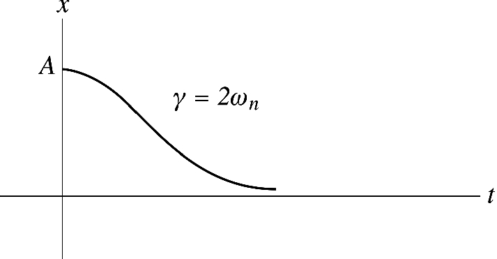
10.4.2 Critically Damped Motion (γ=2ωn)(\gamma =2\omega _{n})

If γ=2ωn\gamma =2\omega _{n}, then the roots are equal real roots

λ1=λ2=γ2=ωn\lambda _{1}=\lambda _{2}=-\frac{\gamma }{2}=-\omega _{n}

In that case, the motion decays without oscillation (see Figure 23) and the general solution of (144) is

x=(C1+C2ωnt)eωntx=(C_{1}+C_{2}\omega _{n}t)e^{-\omega _{n}t}

C1C_{1} and C2C_{2} are found from boundary conditions. If at t=0,x=At=0, x=A, and v=0,v=0, then

x(0)=C1=Ax(0)=C_{1}=A

and

v(0)=ωnC2ωnC1=0v(0)=\omega _{n}C_{2}-\omega _{n}C_{1}=0

or

C1=C2=AC_{1}=C_{2}=A

That gives

x=A(1+ωnt)eωntx=A(1+\omega _{n}t)e^{-\omega _{n}t}
In a critically damped motion, the motion decays without oscillation

Figure 23:In a critically damped motion, the motion decays without oscillation

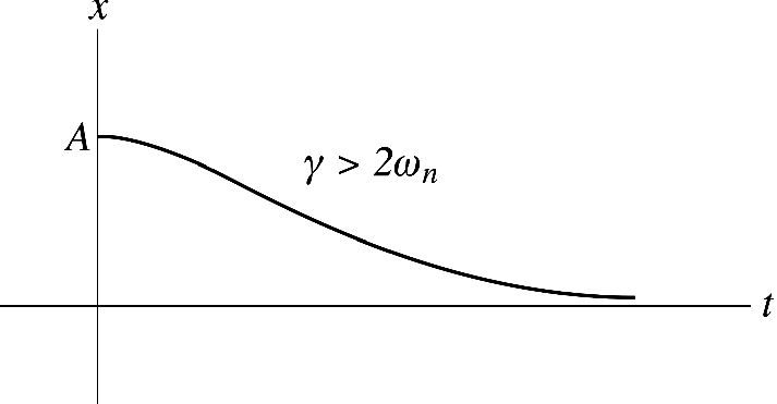
10.4.3 Over Damped Motion (Heavy Damping) (γ>2ωn)(\gamma >2\omega _{n})

If γ>2ωn\gamma >2\omega _{n}, the roots are distinct real roots given by

λ1=γ2+(γ24ωn2)\lambda _{1}=-\frac{\gamma }{2}+\sqrt{\bigg (\frac{\gamma ^{2}}{4}-\omega _{n}^{2}\bigg )}

and

λ2=γ2(γ24ωn2)\lambda _{2}=-\frac{\gamma }{2}-\sqrt{\bigg (\frac{\gamma ^{2}}{4}-\omega _{n}^{2}\bigg )}

The general solution is given by

x=C1eλ1t+C2eλ2tx=C_{1}e^{\lambda _{1}t}+C_{2}e^{\lambda _{2}t}

or

x=(C1eαt+C2eαt)eγ2tx=(C_{1}e^{\alpha t}+C_{2}e^{-\alpha t})e^{-\frac{\gamma }{2}t}

where

α=(γ24ωn2)\alpha =\sqrt{\bigg (\frac{\gamma ^{2}}{4}-\omega _{n}^{2}\bigg )}

C1C_{1} and C2C_{2} are found from boundary conditions. As critical damping, the resulting motion here is nonperiodic but the system returns to its equilibrium position at large values of t unlike critical damping (see Figure 24).

As critical damping, the resulting motion here is non-periodic but the system returns to its equilibrium position at large values of t unlike critical damping

Figure 24:As critical damping, the resulting motion here is non-periodic but the system returns to its equilibrium position at large values of t unlike critical damping

10.4.4 Energy Decay

In damped free vibrations, the total mechanical energy is not constant since the damping force opposes the motion and dissipates the energy of the system. Now, consider the mass–spring system, the total mechanical energy of the system is

E=K+U=12mx˙2+12kx2E=K+U=\frac{1}{2}m\dot{x}^{2}+\frac{1}{2}kx^{2}

The rate of change of energy is

dEdt=(mx¨+kx)x˙\frac{dE}{dt}=(m\ddot{x}+kx)\dot{x}

For damped vibrations in which the damping force is directly proportional to the velocity, we have

mx¨+kx=bx˙m\ddot{x}+kx=-b\dot{x}

Hence,

dEdt=bx˙20\frac{dE}{dt}=-b\dot{x}^{2}\le 0

Thus, the energy decreases with time in any damped motion and the rate in which it decreases is not uniform.

10.5 Forced Vibrations

In the previous sections, only free vibrations have been considered (i.e., vibrations in which only a restoring and damping force act within the system during motion). This section considers the case in which an external driving force is applied to the vibrator. This force is given as a function of time and we have

mx¨+bx˙+kx=F(t)\begin{aligned} m\ddot{x}+b\dot{x}+kx=F(t) \end{aligned}

Here, we will consider the case in which the force is a simple periodic force given by

F(t)=F0cosωt\begin{aligned} F(t)=F_{0}\cos \omega t \end{aligned}

where F0F_{0} is the amplitude and ω\omega is the driving frequency. This force does positive work on the system to balance the energy loss due to damping. Substituting (188) into (187) gives

mx¨+bx˙+kx=F0cosωt\begin{aligned} m\ddot{x}+b\dot{x}+kx=F_{0}\cos \omega t \end{aligned}

or

x¨+γx˙+ωn2x=F0cosωtm\ddot{x}+\gamma \dot{x}+\omega _{n}^{2}x=\frac{F_{0}\cos \omega t}{m}

Let us assume that the solution of (187) is given by

x=C1cosωt+C2sinωtx=C_{1}\cos \omega t+C_{2}\sin \omega t

then, we have

x˙=ωC1sinωt+ωC2cosωt\dot{x}=-\omega C_{1}\sin \omega t+\omega C_{2}\cos \omega t

and

x¨=ω2C1cosωtω2C2sinωt\ddot{x}=-\omega ^{2}C_{1}\cos \omega t-\omega ^{2}C_{2}\sin \omega t

Substituting into (187) gives

(ω2C1cosωtω2C2sinωt)+γ(ωC1sinωt+ωC2cosωt)+ωn2(C1cosωt+C2sinωt)=F0cosωtm\begin{aligned}&(-\omega ^{2}C_{1}\cos \omega t-\omega ^{2}C_{2}\sin \omega t)+\gamma (-\omega C_{1}\sin \omega t+\omega C_{2}\cos \omega t) \nonumber \\&+\omega _{n}^{2}(C_{1}\cos \omega t+C_{2}\sin \omega t)=\frac{F_{0}\cos \omega t}{m} \end{aligned}

That gives

ω2C1+γωC2+ωn2C1=F0m-\omega ^{2}C_{1}+\gamma \omega C_{2}+\omega _{n}^{2}C_{1}=\frac{F_{0}}{m}

and

ω2C2γωC1+ωn2C2=0-\omega ^{2}C_{2}-\gamma \omega C_{1}+\omega _{n}^{2}C_{2}=0

Solving for C1C_{1} and C2C_{2} gives

C1=(F0/m)(ωn2ω2)(ω2ωn2)2+γ2ω2C_{1}=\frac{({F_{0}}/{m})(\omega _{n}^{2}-\omega ^{2})}{(\omega ^{2}-\omega _{n}^{2})^{2}+\gamma ^{2}\omega ^{2}}

and

C2=(F0/m)γω(ω2ωn2)2+γ2ω2C_{2}=\frac{({F_{0}}/{m})\gamma \omega }{(\omega ^{2}-\omega _{n}^{2})^{2}+\gamma ^{2}\omega ^{2}}

Hence,

x=(F0/m)[(ωn2ω2)cosωt+γωsinωt](ω2ωn2)2+γ2ω2x=\frac{({F_{0}}/{m})[(\omega _{n}^{2}-\omega ^{2})\cos \omega t+\gamma \omega \sin \omega t]}{(\omega ^{2}-\omega _{n}^{2})^{2}+\gamma ^{2}\omega ^{2}}

The term in brackets is of the form A1cosωt+A2sinωtA_{1}\cos \omega t+A_{2}\sin \omega t and thus it can be written as Acos(ωtϕ)A'\cos (\omega t-\phi ) where

A=A12+A22A'=\sqrt{A_{1}^{2}+A_{2}^{2}}

i.e.,

A=((ωn2ω2)2+γ2ω2)12A'=((\omega _{n}^{2}-\omega ^{2})^{2}+\gamma ^{2}\omega ^{2})^{\frac{1}{2}}

and

ϕ=tan1A2A1=tan1γω(ω2ωn2)\phi =\tan ^{-1}\frac{A_{2}}{A_{1}}=\tan ^{-1}\frac{\gamma \omega }{(\omega ^{2}-\omega _{n}^{2})}

where 0ϕπ0\le \phi \le \pi. Hence,

x=(F0/m)(ω2ωn2)2+γ2ω2cos(ωtϕ)\begin{aligned} x=\frac{(^{F_{0}}/_{m})}{\sqrt{(\omega ^{2}-\omega _{n}^{2})^{2}+\gamma ^{2}\omega ^{2}}}\cos (\omega t-\phi ) \end{aligned}

If the driving force is applied for a long time compared with the time that the damped vibration dies out, then the system will eventually vibrate at the same frequency of the deriving force. Therefore, the general solution of (144) is called the transient solution since it approaches zero in a relativity short time whereas (189) is called the steady-state solution where the system oscillates with the same frequency as the deriving force. Therefore, the amplitude of a steady-state vibration is

A=(F0/m)(ω2ωn2)2+γ2ω2A=\frac{({F_{0}}/_{m})}{\sqrt{(\omega ^{2}-\omega _{n}^{2})^{2}+\gamma ^{2}\omega ^{2}}}

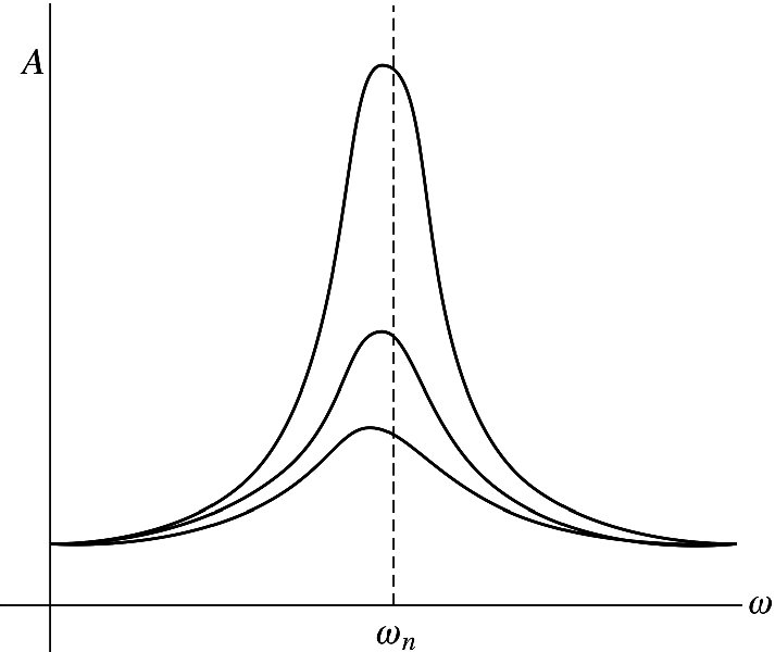
When the deriving frequency ω\omega approaches the natural frequency of the system ωD\omega _{D}, the amplitude of the resulting forced oscillation will increase. This is known as resonance. If the damping is very light, the amplitude reaches its peak when the deriving frequency is nearly equal to the natural frequency ωn\omega _{n}. As the damping becomes heavier, the maximum amplitude shifts to lower frequencies (see Figure 25). In the case where there is no damping at all (b=0)(b=0), the amplitude of resonance is infinite at ω=ωn.\omega =\omega _{n}.

When the deriving frequency \omega approaches the natural frequency of the system \omega _{D}, the amplitude of the resulting forced oscillation will increase. This is known as resonance. If the damping is very light the amplitude reaches its peak when the deriving frequency is nearly equal to the natural frequency \omega _{n}. As the damping becomes heavier, the maximum amplitude shifts to lower frequencies

Figure 25:When the deriving frequency ω\omega approaches the natural frequency of the system ωD\omega _{D}, the amplitude of the resulting forced oscillation will increase. This is known as resonance. If the damping is very light the amplitude reaches its peak when the deriving frequency is nearly equal to the natural frequency ωn\omega _{n}. As the damping becomes heavier, the maximum amplitude shifts to lower frequencies

Problems

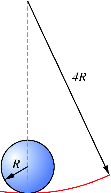
A uniform solid cylinder of radius R and mass M rolls without slipping on a track of radius 4R

Figure 26:A uniform solid cylinder of radius R and mass M rolls without slipping on a track of radius 4R
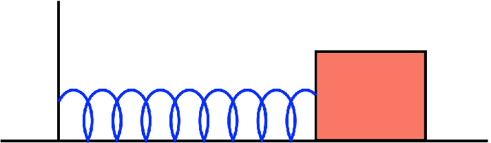
A damped oscillator

Figure 27:A damped oscillator

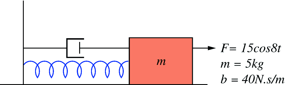
A forced oscillator

Figure 28:A forced oscillator