Mechanics is the science that studies the motion of objects and can be divided into the following:
Kinematics: Describes how objects move in terms of space and time.
Dynamics: Describes the cause of the object’s motion.
Statics: Deals with the conditions under which an object subjected to various forces is in equilibrium.
This chapter is considered with kinematics which answers many questions such as: How long it takes for an apple to reach the ground when it falls from a tree? What is the maximum height reached by a baseball when thrown into air? What is the distance it takes an airplane to take off?
In physics, there are three types of motion: translational, rotational, and vibrational. A block sliding on a surface is in translational motion, a (Merry-go-Round) is an example of rotational motion, and a mass–spring system when stretched and released is in vibrational motion. From here until Chap. 7. Rotation of Rigid Bodies, the object studied will be treated as a particle (i.e., a point mass with no size). This assumption is possible only if the object moves in translational motion without rotating and by neglecting any internal motions that might exist in the object.
That is, an object can be treated as a particle only if all of its parts move in exactly the same way.
For example, if a man jumps into a pool without rotating by doing a somersault (freezing his body), he can be treated as a particle since all particles in his body will move in exactly the same way. Another example of an object that can be treated as a particle is the Earth in its motion about the Sun. Since the dimensions of the Earth are small compared to the dimensions of its path, it can be considered as a particle. The motion of an object is described either by equations or by graphs. Both ways provide information about the motion; however, equations provide precise information while graphs give greater insight about the motion.
This section will discuss the concepts of displacement, velocity, and acceleration in one dimension. These concepts are essential in analyzing the motion of an object.
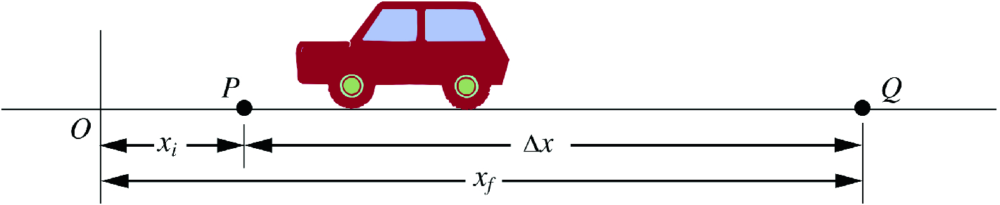
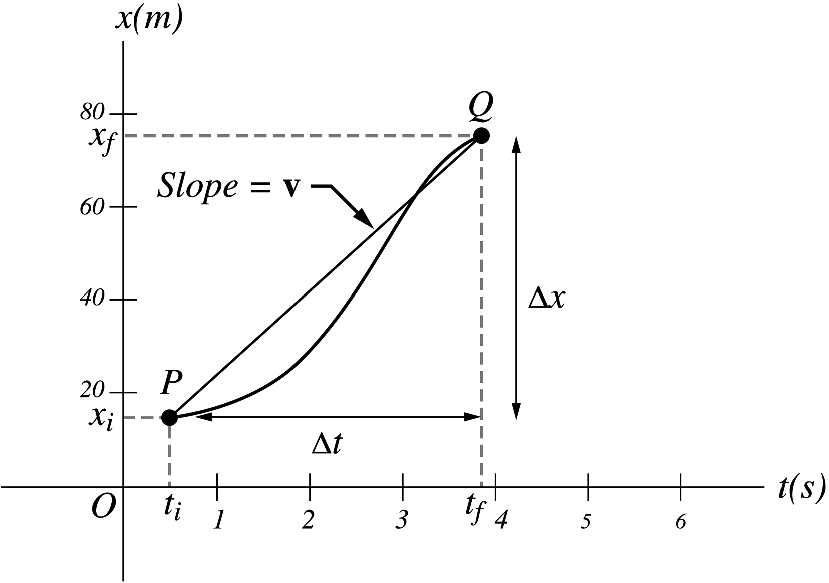
Consider a car that is treated as a particle moving along the straight-line path shown in Figure 1. The x-axis of a coordinate system is used to describe the position of the car with respect to the origin O, where the points P and Q correspond to the positions xi at ti and xf at tf, respectively. The position–time graph of this motion is shown in Figure 2. The displacement of the truck is a vector quantity defined as the change in its position during the time interval from ti to tf and is given by
Hence displacement is a quantity that depends only on the initial and final positions of the object. The direction of the displacement in one dimension is specified by a plus or minus sign. It is positive if the particle is moving in the positive x direction and negative if the particle is moving in the negative x direction. In two or three dimensions, the displacement is represented by a vector. The SI unit of the displacement is the meter (m).
Figure 1:A car that is treated as a particle moving along the straight-line path
Figure 2:The position time graph of the car’s motion
v is positive if the motion is in the positive x-direction and negative if it is in the negative x-direction. On the position–time graph in Figure 2, v is the slope of the straight line connecting the points P and Q. The average velocity helps in describing the overall motion of the particle in a certain time interval. To describe the motion in more detail, the instantaneous velocity is defined. This velocity corresponds to the velocity of a particle at a particular time. That involves allowing △t to approach zero:
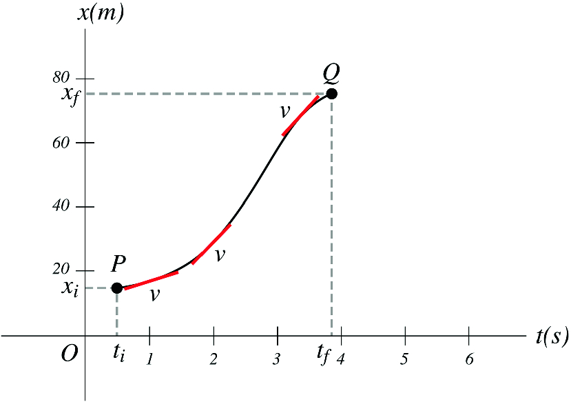
Geometrically, the instantaneous velocity of a particle at a particular time on the position–time curve is the slope (the tangent) to the position–time curve at that point or instance (see Figure 3). The SI unit of the velocity is m/s.
Figure 3:Geometrically, the instantaneous velocity of a particle at a particular time on the position-time curve is the slope (the tangent) to the position-time curve at that point or instance
The speed of the particle is defined as the magnitude of its velocity. Note that speed and average speed are different since speed is defined in terms of displacement, whereas average speed is defined in terms of the total distance traveled.
If the particle’s velocity changes with time, it is said to be accelerating. The average acceleration a of the particle is defined as the ratio of the change of its velocity △v to the time interval △t:
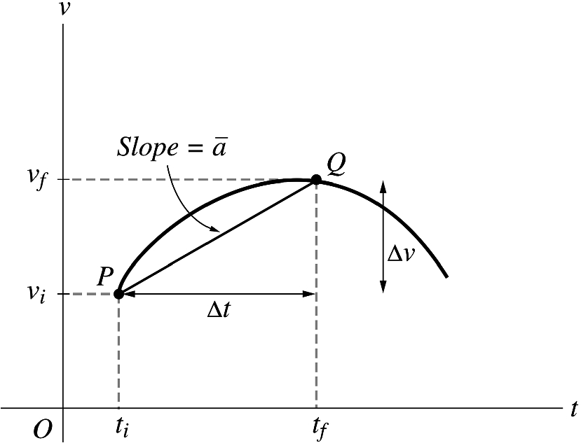
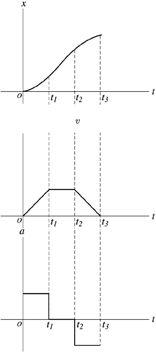
The average acceleration is the slope of the line joining the points P and Q on the velocity–time graph, whereas the instantaneous acceleration is the slope of the curve at a particular point (see Figure 4). Figure 5 shows the position, velocity, and acceleration for a particle simultaneously.
Figure 4:The average acceleration is the slope of the line joining the points P and Q on the velocity-time graph, whereas the instantaneous acceleration is the slope of the curve at a particular point
Figure 5:This figure shows the position, velocity and acceleration as a function of time of a particle moving in one direction. The particle starts from rest, accelerates to a certain speed, is maintained at that speed for some time, then it decelerates back to rest
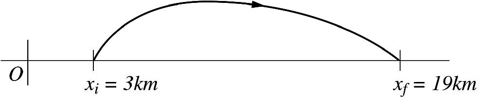
Figure 6:A car moving along the curved path where it is located at xi=3 km at ti=0, and at xf=19 km at tf=0.25 hr
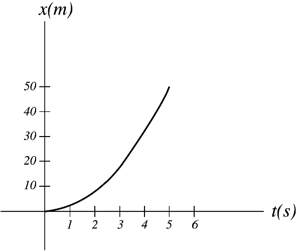
Figure 7:A particle moves along the x-axis according to the expression x=2t2
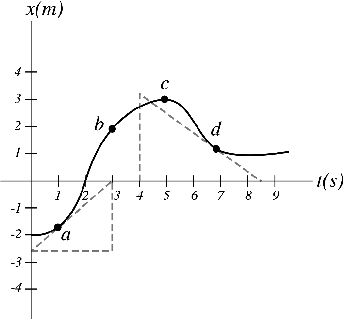
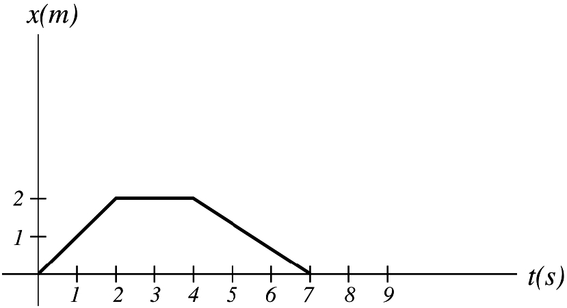
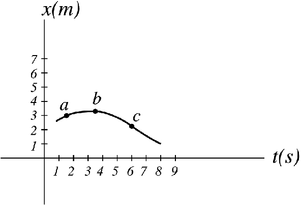
Figure 8:The position-time graph of a particle moving along the x-axis
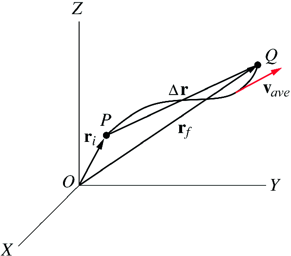
Consider the particle moving from point P to point Q along a path or curve C during a time interval △t=tf−ti as shown in Figure 9. To locate the particle at any point the position vector r=xi+yj+zk is used. ri and rf corresponds to the position vectors of the particle at ti and tf respectively. A position vector should be drawn from a reference point (usually the origin of the coordinate system).
Figure 9:A particle moving from point P to point Q along a path or curve C during a time interval △t=tf−ti
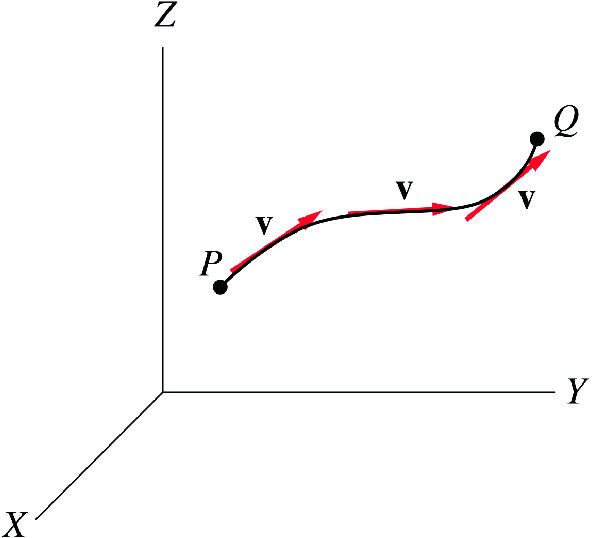
As △t approaches zero, △r becomes tangent to the path and it is replaced by dr. The direction of y is in the direction of dr, hence, y is always tangent to the path at any point. In terms of components y is given by
Figure 10:The instantaneous velocity vectors along the path
where ds is the infinitesimal arc length along the path and comes from the fact that as △t approaches zero, the distance traveled by the particle along the path becomes equal to the vector displacement ∣△r∣. Figure 10 shows the instantaneous velocities along the path. The average acceleration is
Another way to describe motion in three dimensions is by using spherical or cylindrical coordinates. In this book, we will only use rectangular coordinates for three-dimensional motion.
2.3.1 Normal and Tangential Components of Acceleration
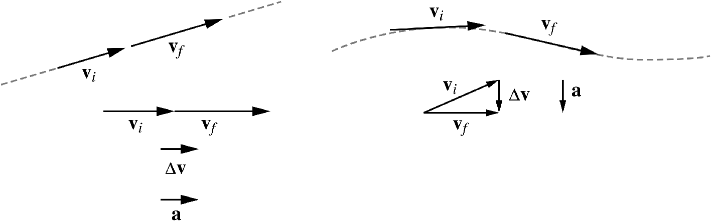
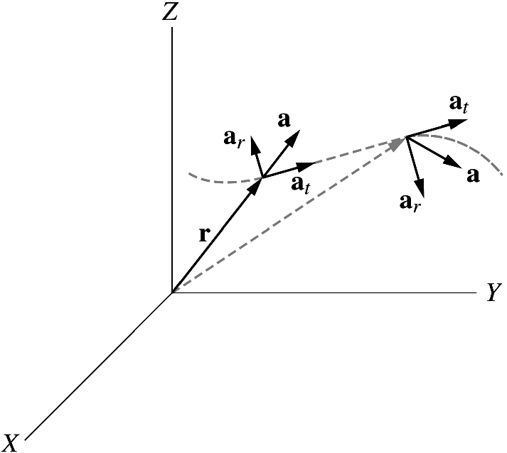
The acceleration describes the change in both the magnitude and direction of the velocity. That is, the acceleration is not necessarily produced due to the change in the magnitude of the velocity only. Sometimes, it is produced due to the change in the direction of the velocity even if its magnitude is unchanged, and sometimes due to the change in both the magnitude and direction. Furthermore, the direction of a is not necessarily in the direction of v. If v is changed in magnitude only (motion along a straight line) then a is parallel to v if v is increasing, and antiparallel if v is decreasing. If v is changed in direction only (motion along a curved path with constant speed), then a is always perpendicular to v at any point (see Figure 11). Finally, if v is changed in both magnitude and direction then a will be directed at some angle to v as in Figure 12.
Figure 11:If v is changed in magnitude only (motion along a straight line) then a is parallel to v if v is increasing, and antiparallel if v is decreasing. If v is changed in direction only (motion along a curved path with constant speed) then a is always perpendicular to v at any point
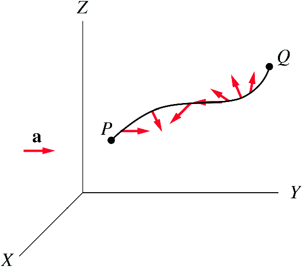
In this case, the acceleration can be resolved into parallel and perpendicular components. The parallel component corresponds to the change in the magnitude of v, while the perpendicular component corresponds to the change in the direction of v. These components can be viewed to be directed along a rectangular coordinate system that moves with the particle (as it moves in space), where the particle is located at the origin of this coordinate system. The parallel (or tangential) component of the acceleration is always tangent to the path while the perpendicular (or normal) component is normal to the path at each point as shown in Figure 13.
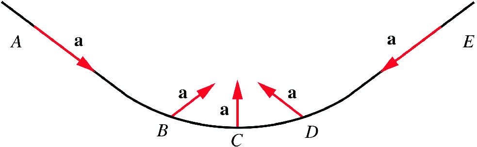
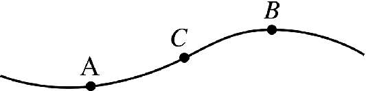
Figure 14 shows the direction of the acceleration of a car moving down a ramp under the influence of gravity.
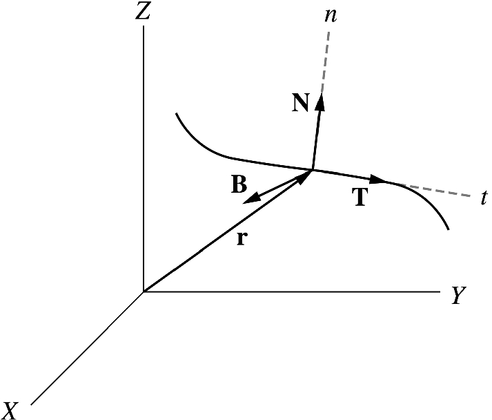
In terms of unit vectors, let T be the unit vector along the tangent axis, N is the unit vector along the normal axis (also called the principal unit normal vector) and B a third unit vector called the binormal vector defined by B=T×N. These unit vectors form a frame called the TNB frame, where it moves with the particle (see Figure 15). Since v is always tangent to the path we may write
Figure 12:If v is changed in both magnitude and direction then a will be directed at some angle to v
Figure 13:The parallel (or tangential) component of the acceleration is always tangent to the path while the perpendicular (or normal) component is normal to the path at each point
Figure 14:At A the acceleration of a car is in the same direction of the velocity since the latter changes only in magnitude. As it moves its velocity is changed in both magnitude and direction. Therefore at B the direction of the acceleration is at some angle to the velocity. At C the speed reaches a maximum and therefore the instantaneous change of speed is zero at this point and the acceleration has only a perpendicular component. As the car moves up its velocity decreases and changes in direction also, thus the acceleration has both parallel and perpendicular components. Finally at E, the acceleration is in the opposite direction of the velocity since the velocity is decreasing but its direction is the same
k is called the curvature of C at a certain point and it has the value k=∣dT/ds∣. The quantity R=1/k is the radius of curvature at that point. Thus, N=R(dT/ds). The total acceleration of the particle in terms of the unit tangent T vector and the principal unit normal vector N can be written as
Therefore, an=v2/R and at=dv/dt. Note that unlike d∣v∣/dt, ∣dv/dt∣ corresponds to the change in the magnitude of the velocity or in its direction or in both (as it represents the magnitude of the total acceleration vector), whereas d∣v∣/dt corresponds to the change in the magnitude only.
2.4.1 One-Dimensional Motion with Constant Acceleration
An acceleration that does not change with time is said to be a constant or uniform acceleration. In that case, the average and instantaneous accelerations are equal. This type of motion is more easily analyzed than when the acceleration is varied. Since the motion is in one dimension, it follows that the y and z components are zero. That is,
Hence, as we’ve mentioned earlier, the direction of the displacement can be specified with a plus or minus sign, as well as the directions of the velocity and acceleration. Let us assume that ti=0, tf=t, vxf=v, vxi=v0, xi=x0 and xf=x. Since the acceleration is constant, the velocity will vary linearly with time, and thus the average velocity can be expressed as
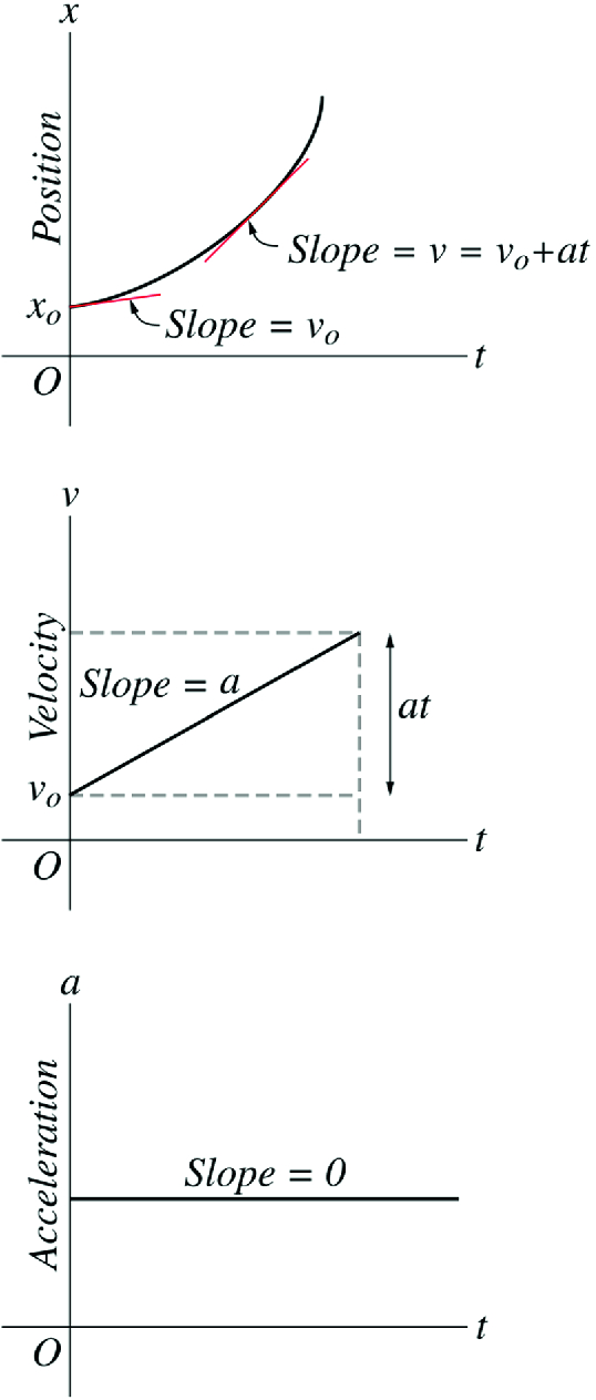
Equations (55), (57), (59), and (61) are called the kinematic equations for motion in a straight line under constant acceleration. The motion graphs for an object moving with constant acceleration in the positive x-direction are shown in Figure 17.
Figure 17:The motion graphs for an object moving with constant acceleration in the positive x-direction
Galileo Galilei (1564–1642) was an Italian scientist, who studied and experimented the acceleration of falling objects. By dropping various objects from the Leaning Tower of Pisa (or by releasing objects from inclined planes according to another story), Galileo discovered that when air resistance is neglected then all objects would fall with the same constant acceleration regardless of their mass or size. This acceleration, denoted by g, is known as the free-fall acceleration since air resistance is neglected and the object is assumed to be moving freely under gravity alone. The direction of the vector g is downwards toward the earth’s center. However, g varies with altitude as well as other factors which will be discussed in Chap. 9. Central Force Motion.
In solving problems involving objects falling near the surface of the earth, g can be assumed to be constant with a value of 9.8 m/s2 and air resistance can be neglected. A free-falling motion is a motion along a straight line (for example along the y-axis) where objects may move upwards or downwards. The kinematics equations of the free-falling motion with constant acceleration can be found from Eqs. ((55)), ((57)), ((59)), and ((61)) by simply replacing x with y and a with g. If the positive direction of y is chosen to be upwards, then the acceleration is negative (downwards) and is given by (a=−g). These substitutions give
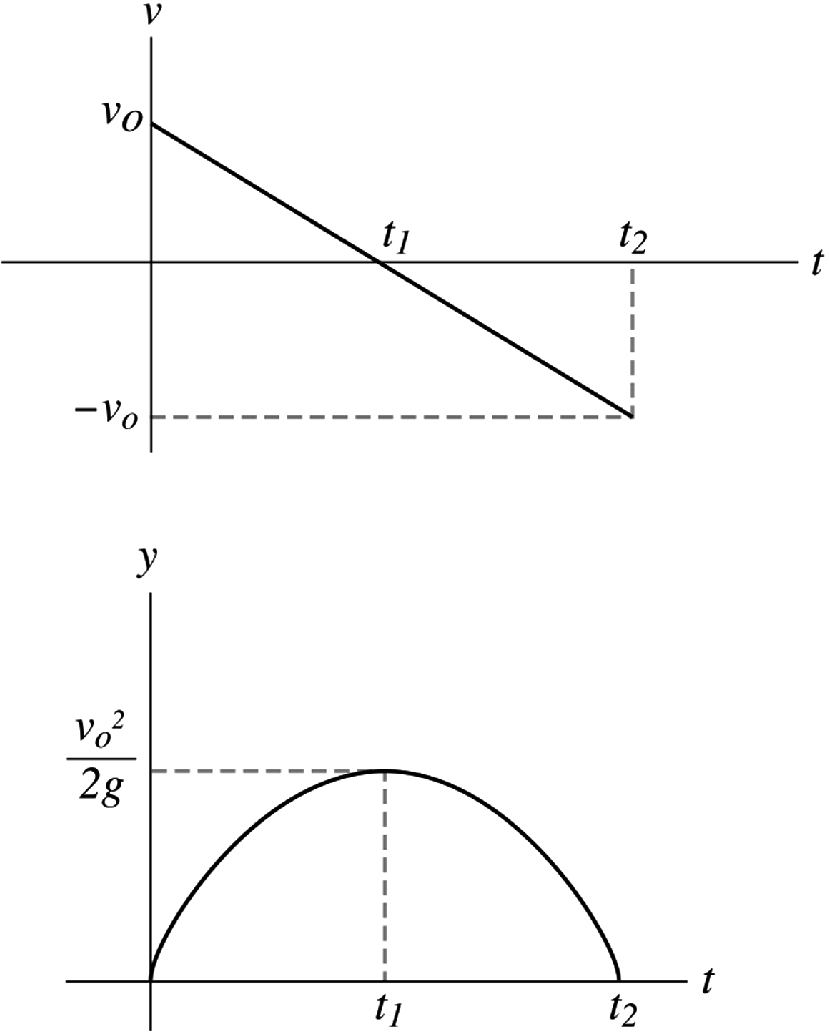
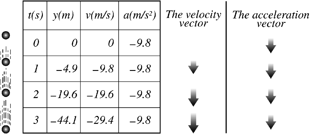
The displacement and velocity graphs are shown in Figure 18. Note that it does not matter whether the object is falling or moving upward, it will experience the same acceleration g which is directed downwards. Figure 19 shows the important features of a free-falling object that is dropped from rest.
Figure 18:The displacement and velocity graph for a free-falling object
Figure 19:The important features of a free falling object that is dropped from rest
2.4.3 Motion in Two Dimensions with Constant Acceleration
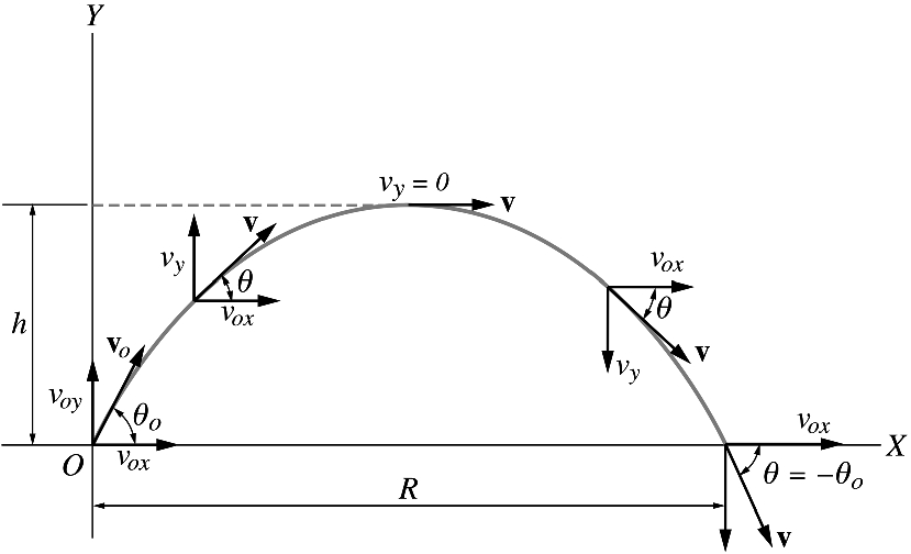
Projectile motion is the motion of an object thrown (projected) into the air at some angle with respect to the surface of the earth, such as the motion of a baseball thrown into the air or an object dropped from a moving airplane. In the simplified model where air resistance as well as other factors such as the Earth’s curvature and rotation are neglected, and if the free-fall acceleration g is assumed constant in magnitude and direction throughout the motion of the object, then the path of the projectile is always a parabola that depends on the magnitude and direction of its initial velocity. Therefore, the projectile can be considered as a combination of a vertical motion with a constant acceleration directed downwards and a horizontal motion with zero acceleration (constant velocity). We can see from Figure 21 that
This equation which is of the form y=ax−bx2 (a and b are constants), is the equation of a parabola. Therefore, when air resistance is neglected (when using the simplified model of the system), the trajectory of the projectile is always a parabola. At any instant, the velocity of the object is tangent to its trajectory Its magnitude and direction with respect to the positive x-direction are given by
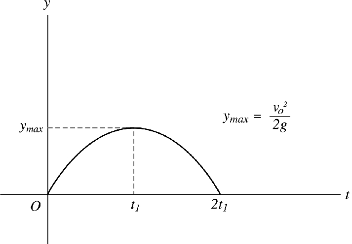
respectively The maximum height h of the projectile, as in Figure 22, is found at t=t1 by noting that at the peak h, vy=0. Substituting this in Eq. (134) gives
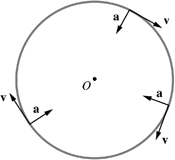
A particle moving in a circular path with constant speed is said to be in uniform circular motion. The motion of the moon about earth, and the motion of clothes in a washing machine are examples of uniform circular motion. In this motion, the direction of the velocity of the particle is continuously changing but its magnitude is constant. As we have mentioned in Sect. 2.3.1 Normal and Tangential Components of Acceleration, when only the direction of the velocity changes, the acceleration is then always perpendicular to the velocity at any time. Therefore, we have only the normal component of the acceleration an=v2/R, and the tangential component of the acceleration at=dv/dt is zero. In the case of the circular path the radius of curvature R is constant, denoted by r, and the normal acceleration is directed along the radius of the circle
The subscript rad is for radial. Thus, this radial or centripetal acceleration arad is always directed toward the center of the circle. Therefore, the directions of v and a change continuously with time but their magnitudes are constant (see Figure 23). The time required for the particle to complete one revolution around the circle is called the period of revolution and is given by
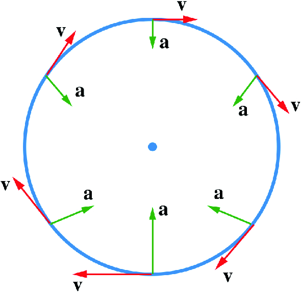
In nonuniform circular motion, the velocity of the particle varies in both magnitude and direction. As mentioned in Sect. 2.3.1 Normal and Tangential Components of Acceleration, when both the magnitude and direction of the particle’s velocity change then its acceleration is directed at some angle to v. Thus, in addition to the normal acceleration in uniform circular motion that corresponds to the change in the direction of v, there is a tangential component that corresponds to the change in the magnitude of v. Furthermore arad is not constant since v changes with time. Therefore, the resultant acceleration is
In Chap. 8. Rolling and Static Equilibrium, the concepts of angular velocity and acceleration and their vector relationship with the normal and tangential accelerations are introduced. Figure 24 shows the velocity and total acceleration vectors of a particle moving in a circular path with increasing speed (clockwise) until it reaches the maximum speed at the bottom, and then slows down as it goes back up. An example of this motion is in a roller coaster ride in a vertical circle.
Figure 24:The velocity and total acceleration vectors of a particle moving in a circular path with increasing speed (clockwise) until it reaches the maximum speed at the bottom, and then slows down as it goes back up. An example of this motion is in a roller coaster ride in a vertical circle
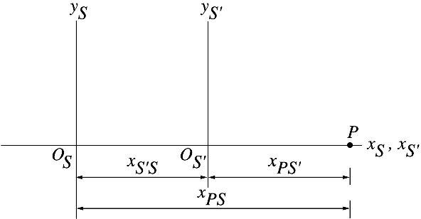
In this section, we will see how observers moving relative to each other obtain different results when measuring the velocity of a moving body. Suppose two cars are moving besides each other at the same speed of 120 km/h with respect to earth. In this case, any of the two cars is at rest relative to the other. According to an observer who is stationary with respect to earth, each car is moving with a speed of 120 km/s. A second observer, in any of the cars, will see the stationary observer moving backwards at a speed of 120 km/h. In addition, if a third car is moving ahead of the two cars at a speed of 140 km/h relative to earth, then its speed relative to an observer in any of the two cars is 20 km/s. Thus, the displacement and velocities may have different values when measured relative to different observers. Therefore, the description of motion depends on the observer. By attaching a coordinate system to an observer together with an appropriate time scale, he or she are then said to be in a reference frame. In measuring quantities, it is essential to specify the reference frame. In most situations, the earth (the lab) is used as our frame of reference. To understand this, consider a particle moving in one dimension in the positive x-direction. Suppose two observers want to describe its motion, one is observer S who is stationary relative to the ground, and the other is observer S′, who is moving in the positive x-direction with a constant velocity relative to the ground (see Figure 25). At any instant, the position of the particle relative to S is xPS, and its position relative to S′ is xPS′. The relation between these two observations is
Therefore, the position of P relative to OS is equal to the position of P relative to OS′ plus the distance between OS and OS′. Differentiating Eq. (167) with respect to time we get
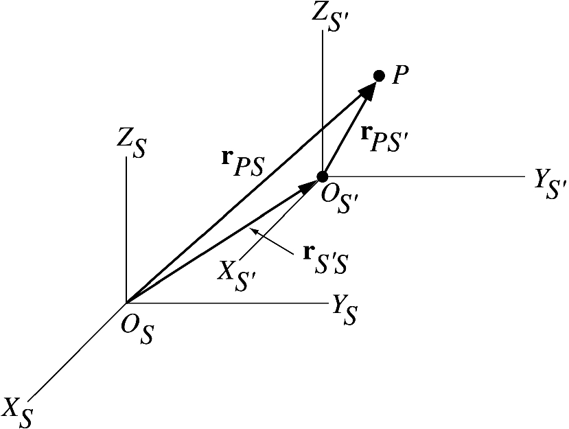
We will extend this to three dimensions in the case where the velocity of S′ with respect to S(vS′S) is constant in both magnitude and direction (see Figure 26). The position vector of the particle P relative to S is given by
Figure 25:Observer S is stationary relative to the ground, and observer S′ is moving in the positive x-direction with a constant velocity relative to the ground
Figure 26:The velocity of S′ with respect to S(vS′S) is constant in both magnitude and direction
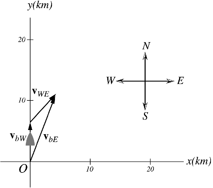
Figure 29:A boat is traveling at 8 km/h north relative to the sea’s waves, and the waves are traveling northeast relative to the earth at a constant speed of 4 km/h
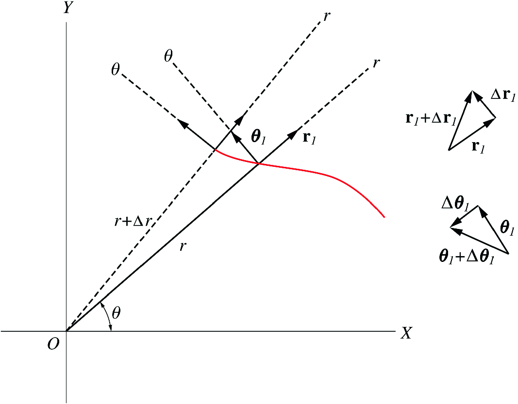
Figure 30:r1 is a unit vector along the increasing r direction and θ1 is a unit vector in the direction of increasing θ (anticlockwise direction)
Consider a particle moving in the x–y plane. A useful way to describe the position, velocity, and acceleration of the particle is by using its polar coordinates (r,θ). The relationship between the polar and rectangular coordinates is
where θ is measured from the positive x- axis. Suppose a particle is located at (r,θ). If the particle moves in a straight line along the r direction, then θ is constant through the motion of the particle. If the particle moves in a circle, then r is constant. Let r1 be a unit vector along the increasing r direction and θ1 to be a unit vector in the direction of increasing θ (anticlockwise direction). From Figure 30, we have
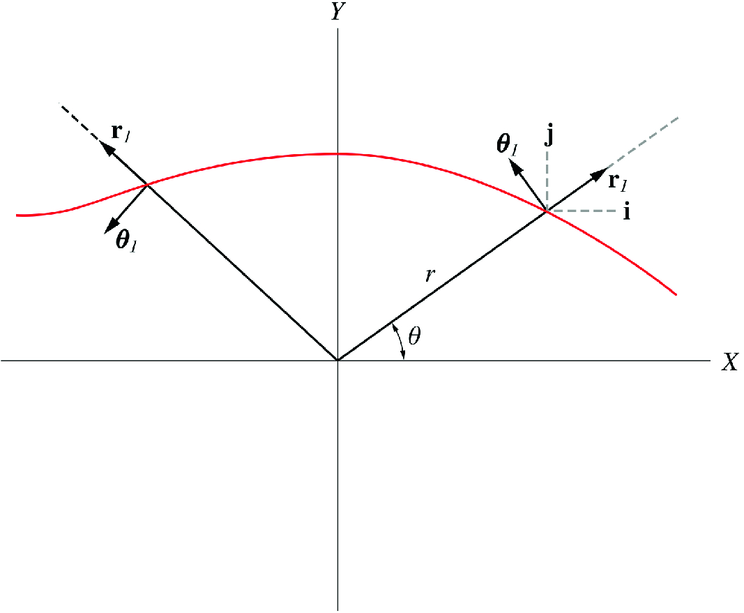
Unlike the rectangular unit vectors, the polar unit vectors are not fixed in direction. Their direction changes as the particle moves along some path. Therefore, when finding the velocity and acceleration of a particle the derivatives of the polar unit vectors must be considered. The position vector of the particle is given by
Figure 31:Unlike the rectangular unit vectors, the polar unit vectors are not fixed in direction. Their direction changes as the particle moves along some path
where vr=r˙ and vθ=rθ˙ and v=vr2+vθ2. The total acceleration is