Skip to article frontmatterSkip to article content
Site not loading correctly?

This may be due to an incorrect BASE_URL configuration. See the MyST Documentation for reference.

1. Units and Vectors

King Abdullah University of Science and Technology

1.1 Introduction

Physics is an exciting adventure that is concerned with unraveling the secrets of nature based on observations and measurements and also on intuition and imagination. Its beauty lies in having few fundamental principles being able to reach out to incorporate many phenomena from the atomic to the cosmic scale. It is a science that depends heavily on mathematics to prove and express theories and laws and is considered to be the most fundamental of physical sciences. Astronomy, geology, and chemistry all involve applications of physics’ principles and concepts. Physics doesn’t only provide theories, but it also provides techniques that are used in every area of life. Modern physical techniques were the major contributors to the wealth of mankind’s knowledge in the past century.

A simple law in physics can be used to explain a wide range of complex phenomena that may appear to be not related. When studying a complex physical system, a simplified model of the system is usually used, where the minor effects are neglected and the main features of the system are concentrated upon. For example, when dealing with an object falling near the earth’s surface, air resistance can be neglected. In addition, the earth is usually assumed to be spherical and homogeneous. However, in reality, the earth is an ellipsoid and is not homogeneous. The difference between the calculations of these different models can be assumed to be insignificant.

Physics can be divided into two branches namely: classical physics and modern physics. This book focuses on mechanics, which is a branch of classical physics. Other branches of classical physics are: light and optics, sound, electromagnetism, and thermodynamics. Mechanics is the science of motion of objects and is the core of classical physics. On the other hand, modern branches of physics include theories that have been developed during the past twentieth century. Two main theories are the theory of relativity and the theory of quantum mechanics. Modern physics explains many physical phenomena that cannot be explained by classical physics.

1.2 The SI Units

A physical quantity is a quantitative description of a physical phenomenon. For a precise description, one has to measure the physical quantity and represent this measurement by a number. Such a measurement is made by comparing the quantity with a standard; this standard is called a unit. For example, mass is a physical quantity that refers to the quantity of matter contained in an object. The unit kilogram is one of the units used to measure mass and is defined as the mass of a specific platinum–iridium alloy cylinder, kept at the International Bureau of Weights and Measures. Therefore, when we say that a block’s mass is 300 kg, we mean that it is 300 times the mass of the cylindrical platinum–iridium alloy. All units chosen should obey certain properties such as being accurate, accessible, and should remain stable under varied environmental conditions or time.

In 1960, the International System of units (SI) (formally known as the Metric System MKS) was established. The abbreviation is derived from the French phrase “System International”. As shown in Table Paragraph, the SI system consists of seven base fundamental units, each representing a quantity assumed to be naturally independent. The system also includes two supplementary units, the radian which is a unit of the plane angle, and the steradian which is a unit of the solid angle. All other quantities in physics are derived from these base quantities. For example, mechanical quantities such as force, velocity, volume, and energy can be derived from the fundamental quantities length, mass, and time. Furthermore, the powers of ten are used to represent the larger and smaller values for a certain physical quantity as listed in Table Paragraph. The most recent definitions of the units of length, mass, and time in the SI system are as follows:

Table 1.1 The SI system consists of seven base fundamental units, each representing a quantity assumed to be naturally independent

QuantityUnit nameUnit symbol
LengthMeterm
MassKilogramkg
TimeSeconds
TemperatureKelvinK
Electric CurrentAmpereA
Luminous IntensityCandelacd
Amount of Substancemolemol

Table 1.2 Prefixes for Powers of Ten

FactorPrefixSymbol
10-24yoctoy
10-21zeptoz
10-18attoa
10-15femtof
10-12picop
10-9nanon
10-6microμ\mu
10-3millim
10-2centic
10-1decid
101dekada
102hectoh
103kilok
106megaM
109gigaG
1012teraT
1015petaP
1018exaE
1021zettaZ

1.3 Conversion Factors

There are two other major systems of units besides the SI units. The (CGS) system of units which uses the centimeter, gram and second as its base units, and the (FPS) system of units which uses the foot, pound, and second as its base units. The conversion factors between the SI units and other systems of units of length, mass, and time are

1.4 Dimension Analysis

The symbols used to specify the dimensions of length, mass, and time are L,M\mathrm{L}, \mathrm{M} and T\mathrm{T}, respectively. Dimension analysis is a method used to check the validity of an equation and to derive correct expressions. Only the same dimensions can be added or subtracted, i.e., they obey the rules of algebra. To check the validity of an equation, the terms on both sides must have the same dimension. The dimension of a physical quantity is denoted using brackets [ ]. For example, the dimension of the volume is [V]=L3[V]=\mathrm{L}^{3}, and that of acceleration is [a]=L/T3[\mathrm{a}]=\mathrm{L}/\mathrm{T}^{3}

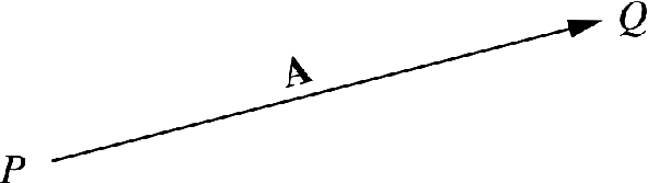
A vector is represented geometrically by an arrow PQ drawn to scale

Figure 1:A vector is represented geometrically by an arrow PQ drawn to scale

1.5 Vectors

When exploring physical quantities in nature, it is found that some quantities can be completely described by giving a number along with its unit, such as the mass of an object or the time between two events. These quantities are called scalar quantities. It is also found that other quantities are fully described by giving a number along with its unit in addition to a specified direction, such as the force on an object. These quantities are called vector quantities.

Scalar quantities have magnitude but don’t have a direction and obey the rules of ordinary arithmetic. Some examples are mass, volume, temperature, energy, pressure, and time intervals by a letter such as m, t, E \ldots, etc. Vector quantities have both magnitude and direction and obey the rules of vector algebra. Examples are displacement, force, velocity, and acceleration. Analytically, a vector is specified by a bold face letter such as A\mathbf{A}. This notation (as used in this book) is usually used in printed material. In handwriting, the designation A\overrightarrow{A} is used. The magnitude of A\mathbf{A} is written as A|\mathbf{A}| or A in print or as A|\overrightarrow{A}| in handwriting.

A vector is represented geometrically by an arrow PQ drawn to scale as shown in Figure 1. The length and direction of the arrow represent the magnitude and direction of the vector, respectively, and is independent of the choice of coordinate system. The point P\mathrm{P} is called the initial point (tail of A) and Q\mathrm{Q} is called the terminal point (head of A).

1.6 Vector Algebra

In this section, we will discuss how mathematical operations are applied to vectors.

1.6.1 Equality of Two Vectors

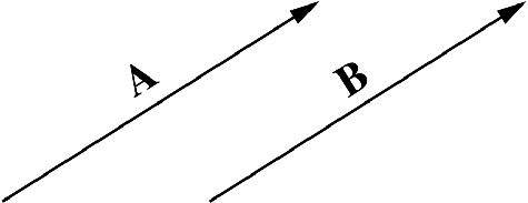
The two vectors A\mathbf{A} and B\mathbf{B} are said to be equal (A=B)(\mathbf{A}=\mathbf{B}) only if they have the same magnitude and direction, whether or not their initial points are the same as shown in Figure 2.

The two vectors \mathbf{A} and \mathbf{B} are said to be equal (\mathbf{A} = \mathbf{B}) only if they have the same magnitude and direction

Figure 2:The two vectors A\mathbf{A} and B\mathbf{B} are said to be equal (A\mathbf{A} = B\mathbf{B}) only if they have the same magnitude and direction

1.6.2 Addition

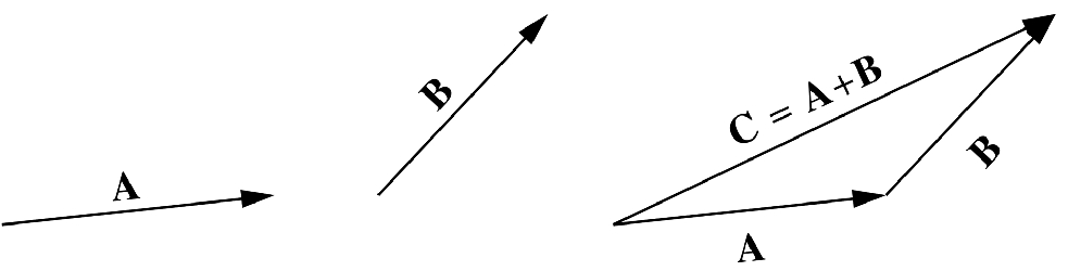
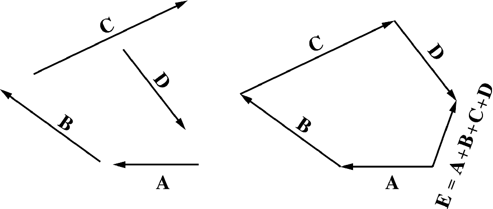
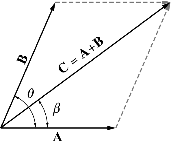
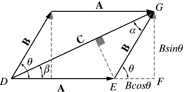
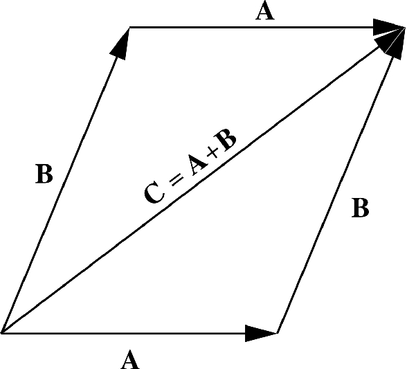
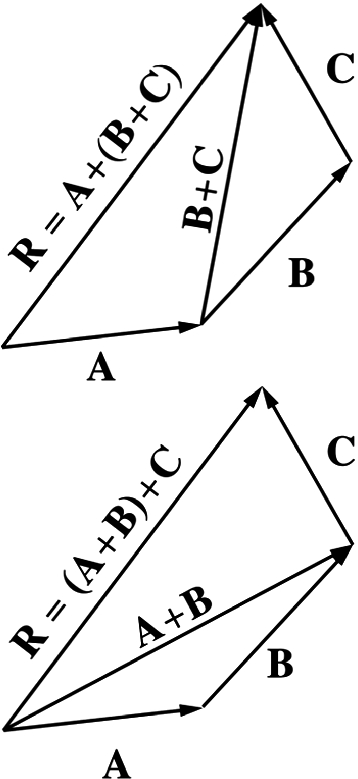
There are two ways to add vectors, geometrically and algebraically. Here, we will discuss the geometric method which is useful for solving problems without using a coordinate system. The algebraic method will be discussed later. To add two vectors A\mathbf{A} and B\mathbf{B} using the geometric method, place the head of A\mathbf{A} at the tail of B\mathbf{B} and draw a vector from the tail of A\mathbf{A} to the head of B\mathbf{B} as shown in Figure 3. This method is known as the triangle method. An extension to sum up more than two vectors is shown in Figure 4. An alternative procedure of vector addition using the geometric method is shown in Figure 5. This is known as the parallelogram method, where C\mathbf{C} is the diagonal of a parallelogram with sides A and B. To find C\mathbf{C} analytically, Figure 6 shows that

(DG)2=(DF)2+(FG)2(DG)^{2}=(DF)^{2}+(FG)^{2}

and that

DF=DE+EF=A+Bcosθ,DF=DE+EF=A+B\cos \theta ,

Thus, Eq. (6) becomes

C2=(A+Bcosθ)2+(Bsinθ)2=A2+B2+2ABcosθ,C^{2}=(A+B\cos \theta )^{2}+(B\sin \theta )^{2}=A^{2}+B^{2}+2AB\cos \theta ,
To add two vectors \mathbf{A} and \mathbf{B} using the geometric method, place the head of \mathbf{A} at the tail of \mathbf{B} and draw a vector from the tail of \mathbf{A} to the head of \mathbf{B}

Figure 3:To add two vectors A\mathbf{A} and B\mathbf{B} using the geometric method, place the head of A\mathbf{A} at the tail of B\mathbf{B} and draw a vector from the tail of A\mathbf{A} to the head of B\mathbf{B}

Geometric method for summing more than two vectors

Figure 4:Geometric method for summing more than two vectors

The parallelogram method of adding two vectors

Figure 5:The parallelogram method of adding two vectors

Finding the magnitude and the direction of \mathbf{C}

Figure 6:Finding the magnitude and the direction of C\mathbf{C}

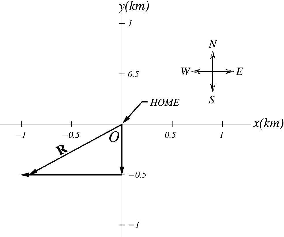
The total displacement of the jogger is the vector \mathbf{R}

Figure 7:The total displacement of the jogger is the vector R\mathbf{R}

or

C=A2+B2+2ABcosθ,C=\sqrt{A^{2}+B^{2}+2AB\cos \theta },

The direction of C\mathbf{C} is

tanβ=GFDF=GFDE+EF=BsinθA+Bcosθ,\tan \beta =\frac{GF}{DF}=\frac{GF}{DE+EF}=\frac{B\sin \theta }{A+B\cos \theta },

Note that only when A\mathbf{A} and B\mathbf{B} are parallel, the magnitude of the resultant vector C\mathbf{C} is equal to A+BA+B (unlike the addition of scalar quantities, the magnitude of the resultant vector C\mathbf{C} is not necessarily equal to A+BA+B).

1.6.3 Negative of a Vector

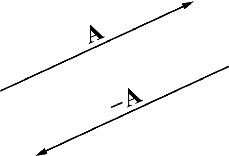
The negative vector of A\mathbf{A} is a vector of the same magnitude of A\mathbf{A} but in the opposite direction as shown in Figure 8, and it is denoted by A-\mathbf{A}.

The negative vector of \mathbf{A} is a vector of the same magnitude of \mathbf{A} but in the opposite direction

Figure 8:The negative vector of A\mathbf{A} is a vector of the same magnitude of A\mathbf{A} but in the opposite direction

1.6.4 The Zero Vector

The zero vector is a vector of zero magnitude and has no defined direction. It may result from A=BB=0\mathbf{A}=\mathbf{B}-\mathbf{B}=\mathbf{0} or from A=cB=0\mathbf{A}=c\mathbf{B}=0 if c=0.c=0.

1.6.5 Subtraction of Vectors

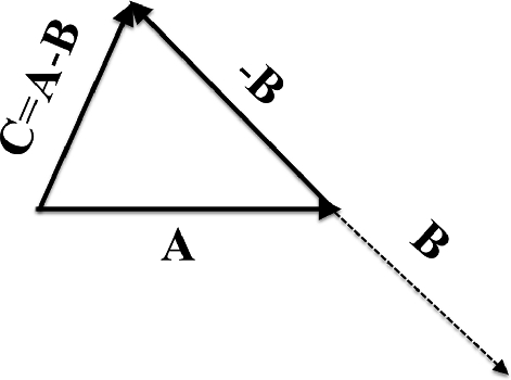
The vector AB\mathbf{A}-\mathbf{B} is defined as the vector that when added to B\mathbf{B} gives us A\mathbf{A}. Equivalently, AB\mathbf{A}-\mathbf{B} can be defined as the vector A\mathbf{A} added to vector B-\mathbf{B} (A+(B))(\mathbf{A}+(-\mathbf{B})) as shown in Figure 9.

Subtraction of two vectors

Figure 9:Subtraction of two vectors

1.6.6 Multiplication of a Vector by a Scalar

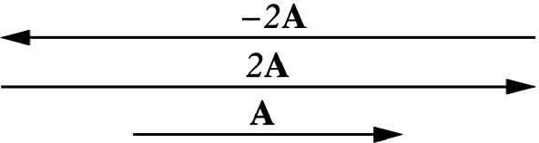
The product of a vector A\mathbf{A} by a scalar q is a vector qAq\mathbf{A} or Aq\mathbf{A}q. Its magnitude is qA and its direction is the same as A\mathbf{A} if q is positive and opposite to A\mathbf{A} if q is negative, as shown in Figure 10.

The product of a vector by a scalar

Figure 10:The product of a vector by a scalar

Commutative law of addition

Figure 11:Commutative law of addition

Associative law of addition

Figure 12:Associative law of addition

1.6.7 Some Properties

1.6.8 The Unit Vector

The unit vector is a vector of magnitude equal to 1, and with the same direction of A\mathbf{A}. For every A0,a=A/A\mathbf{A}\ne 0, \mathbf{a}=\mathbf{A}/|\mathbf{A}| is a unit vector.

1.6.9 The Scalar (Dot) Product

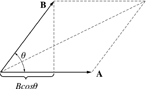
The scalar product is a scalar quantity defined as AB=ABcosθ\mathbf{A}\cdot \mathbf{B}=AB\cos \theta, where θ\theta is the smaller angle between A\mathbf{A} and B\mathbf{B} (0θπ)(0\le \theta \le \pi ) (see Figure 13).

The scalar product of two vectors

Figure 13:The scalar product of two vectors

Some Properties of the Scalar Product

1.6.10 The Vector (Cross) Product

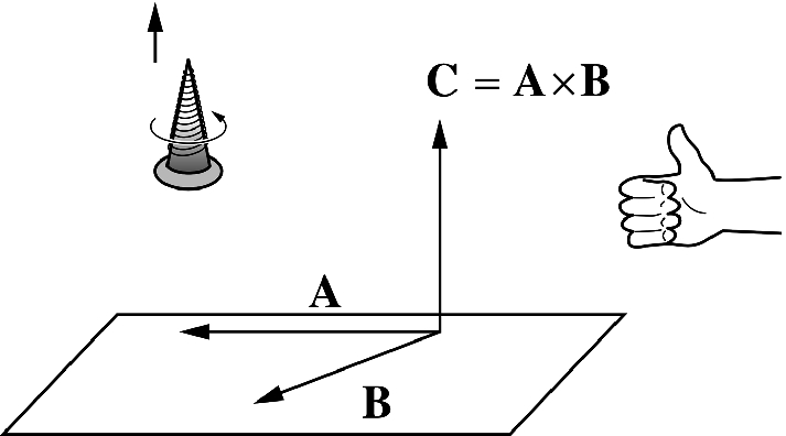
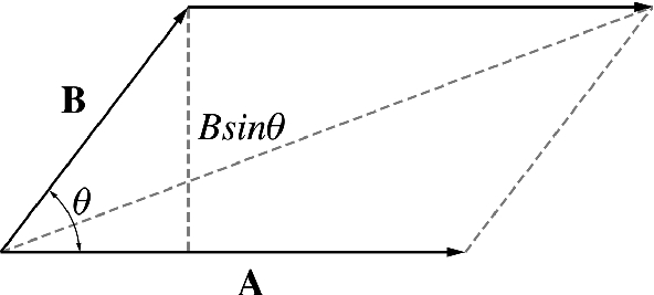
The vector product is a vector quantity defined as C=A×B\mathbf{C}=\mathbf{A}\times \mathbf{B} (read A cross B) with magnitude equal to A×B=ABsinθ,(0θπ)|\mathbf{A}\times \mathbf{B}|=AB\sin \theta , (0\le \theta \le \pi ). The direction of C\mathbf{C} is found from the right-hand rule or of advance of a right-handed screw rotated from A\mathbf{A} to B\mathbf{B} as shown in Figure 14. C\mathbf{C} is perpendicular to the plane formed by A\mathbf{A} and B\mathbf{B}.

The vector product of two vectors

Figure 14:The vector product of two vectors

Some Properties

The magnitude of the vector product |\mathbf{A}\times \mathbf{B}| is the area of a parallelogram with sides A and B

Figure 15:The magnitude of the vector product A×B|\mathbf{A}\times \mathbf{B}| is the area of a parallelogram with sides AA and BB

1.7 Coordinate Systems

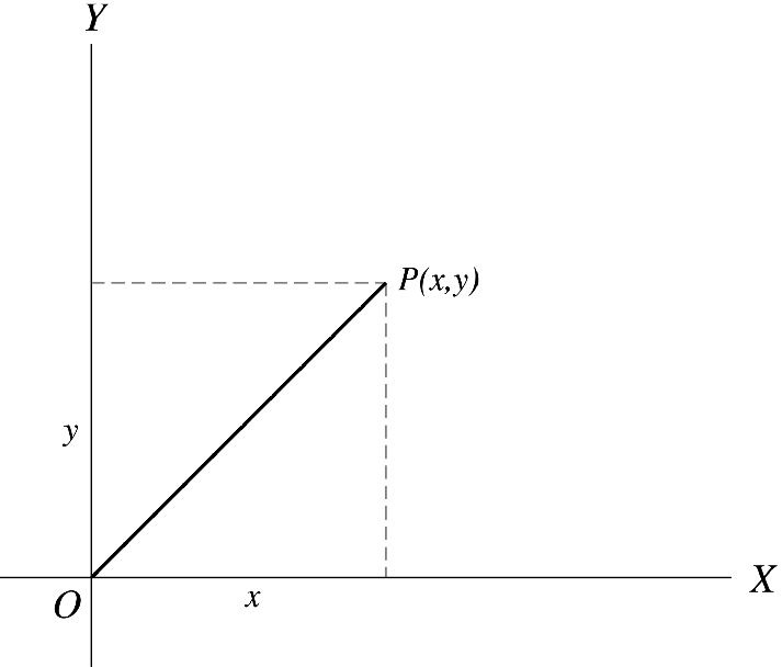
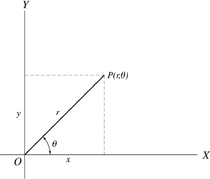
To specify the location of a point in space, a coordinate system must be used. A coordinate system consists of a reference point called the origin O\mathrm{O} and a set of labeled axes. The positive direction of an axis is in the direction of increasing numbers, whereas the negative direction is opposite. Figures Figure 16 and Figure 17 show the rectangular (or Cartesian) coordinate system and the polar coordinates of a point, respectively The rectangular coordinates x and y are related to the polar coordinates r and θ\theta by the following relations:

x=rcosθx=r\cos \theta
y=rsinθy=r\sin \theta
tanθ=y/x\tan \theta =y/x
r=x2+y2r=\sqrt{x^{2}+y^{2}}

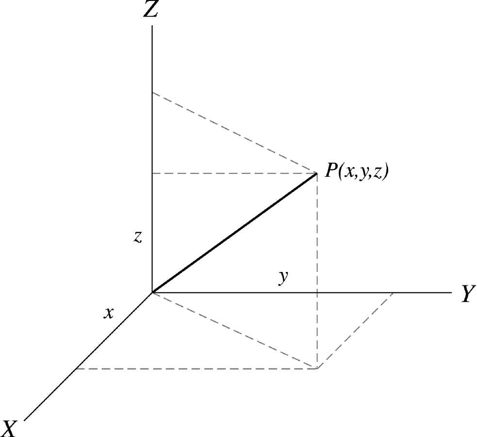
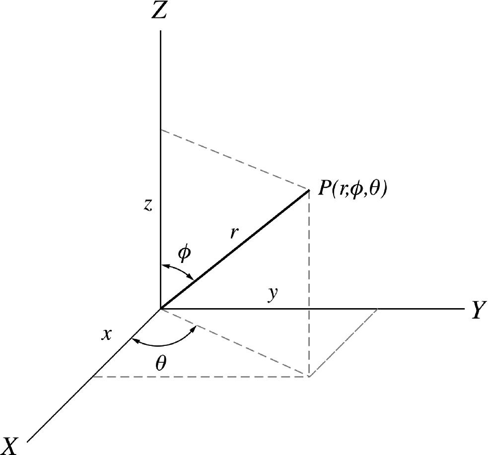
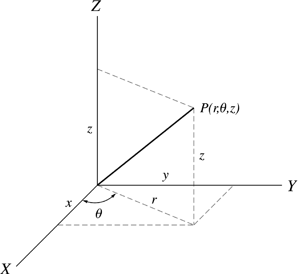
In three dimensions, the cartesian coordinate system is shown in Figure 18. Other used coordinate systems in three dimensions are the spherical and cylindrical coordinates (Figure 19 and Figure 20).

The rectangular (cartesian) coordinate system

Figure 16:The rectangular (cartesian) coordinate system

The polar coordinate system

Figure 17:The polar coordinate system

The cartesian coordinate system in three dimensions

Figure 18:The cartesian coordinate system in three dimensions

The spherical coordinate system

Figure 19:The spherical coordinate system

The cylindrical coordinate system

Figure 20:The cylindrical coordinate system

1.8 Vectors in Terms of Components

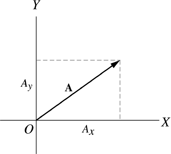
In two dimensions, the vector A\mathbf{A} can be expressed as the sum of two other vectors A=Ax+Ay\mathbf{A}=\mathbf{A}_{x}+\mathbf{A}_{y}, where Ax=AcosθA_{x}=A\cos \theta and Ay=AsinθA_{y}=A\sin \theta as shown in Figure 21.

In two dimensions, the vector \mathbf{A} can be expressed as the sum of two other vectors \mathbf{A}=\mathbf{A}_{x}+\mathbf{A}_{y}, where A_{x}=A\cos \theta and A_{y}=A\sin \theta

Figure 21:In two dimensions, the vector A\mathbf{A} can be expressed as the sum of two other vectors A=Ax+Ay\mathbf{A}=\mathbf{A}_{x}+\mathbf{A}_{y}, where Ax=AcosθA_{x}=A\cos \theta and Ay=AsinθA_{y}=A\sin \theta

Ax\mathbf{A}_{x} and Ay\mathbf{A}_{y} are called the rectangular components, or simply components of A\mathbf{A} in the x\mathrm{x} and y\mathrm{y} directions respectively The magnitude and direction of A\mathbf{A} are related to its components through the expressions:

A=Ax2+Ay2A=\sqrt{A_{x}^{2}+A_{y}^{2}}
tanθ=Ay/Ax\tan \theta =A_{y}/A_{x}

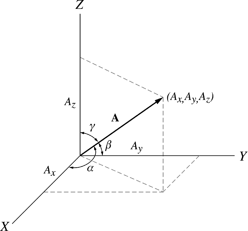
In three dimensions (see Figure 22), the magnitude of A is given by

A=Ax2+Ay2+Az2A=\sqrt{A_{x}^{2}+A_{y}^{2}+A_{z}^{2}}

with directions given by

cosα=Ax/A, cosβ=Ay/A, cosγ=Az/A\cos \alpha =A_{x}/A,\ \cos \beta =A_{y}/A,\ \cos \gamma =A_{z}/A
In three dimensions the magnitude of A is A=\sqrt{A_{x}^{2}+A_{y}^{2}+A_{z}^{2}}

Figure 22:In three dimensions the magnitude of A is A=Ax2+Ay2+Az2A=\sqrt{A_{x}^{2}+A_{y}^{2}+A_{z}^{2}}

1.8.1 Rectangular Unit Vectors

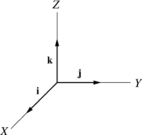
The rectangular unit vectors i,j\mathbf{i}, \mathbf{j}, and k\mathbf{k} are unit vectors defined to be in the direction of the positive x\mathrm{x}-, y\mathrm{y}-, and z\mathrm{z}-axes, respectively, of the rectangular coordinate system as shown in Figure 23. Note that labeling the axes in this way forms a right-handed system. This name derives from the fact that a right- handed screw rotated through 9090^{\circ} from the x\mathrm{x}-axis into the y\mathrm{y}-axis will advance in the positive z\mathrm{z}-direction. (Note that throughout this book the right-handed coordinate system is used). In terms of unit vectors, vector A can be written as

A=Axi+Ayj+Azk\mathbf{A}=A_{x}\mathbf{i}+A_{y}\mathbf{j}+A_{z}\mathbf{k}
The rectangular unit vectors \mathbf{i}, \mathbf{j} and \mathbf{k} are unit vectors defined to be in the direction of the positive \mathrm{x}, \mathrm{y}, and \mathrm{z} axes respectively

Figure 23:The rectangular unit vectors i,j\mathbf{i}, \mathbf{j} and k\mathbf{k} are unit vectors defined to be in the direction of the positive x,y\mathrm{x}, \mathrm{y}, and z\mathrm{z} axes respectively

1.8.2 Component Method

Suppose we have A=Axi+Ayj\mathbf{A}=A_{x}\mathbf{i}+A_{y}\mathbf{j} and B=Bxi+Byj\mathbf{B}=B_{x}\mathbf{i}+B_{y}\mathbf{j}

Addition

The resultant vector C\mathbf{C} is given by

C=A+B=(Ax+Bx)i+(Ay+By)j=Cxi+Cyj\mathbf{C}=\mathbf{A}+\mathbf{B}=(A_{x}+B_{x})\mathbf{i}+(A_{y}+B_{y})\mathbf{j}=C_{x}\mathbf{i}+C_{y}\mathbf{j}
Cx=Ax+BxC_{x}=A_{x}+B_{x}
Cy=Ay+ByC_{y}=A_{y}+B_{y}

Thus, the magnitude of C\mathbf{C} is

C=Cx2+Cy2C=\sqrt{C_{x}^{2}+C_{y}^{2}}

with a direction

tanθ=CyCx=Ay+ByAx+Bx\tan \theta =\frac{C_{y}}{C_{x}}=\frac{A_{y}+B_{y}}{A_{x}+B_{x}}

in three dimensions

C=(Ax+Bx)i+(Ay+By)j=(Az+Bz)k=Cxi+Cyj+Czk\mathbf{C}=(A_{x}+B_{x})\mathbf{i}+(A_{y}+B_{y})\mathbf{j}=(A_{z}+B_{z})\mathbf{k}=C_{x}\mathbf{i}+C_{y}\mathbf{j}+C_{z}\mathbf{k}

the magnitude of C\mathbf{C} is

C=Cx2+Cy2+Cz2C=\sqrt{C_{x}^{2}+C_{y}^{2}+C_{z}^{2}}

And the directions are

cosα=Cx/C,  cosβ=Cy/C,  cosγ=Cz/C\cos \alpha =C_{x}/C, \; \cos \beta =C_{y}/C, \; \cos \gamma =C_{z}/C

This component method is easy to use in adding any number of vectors.

Subtraction

C=AB=(AxBx)i+(AyBy)j+(AzBz)k{\mathbf{C}}={\mathbf{A}}-{\mathbf{B}}=(A_{x}-B_{x})\mathbf{i}+(A_{y}-B_{y})\mathbf{j}+(A_{z}-B_{z})\mathbf{k}

The magnitude and direction of C\mathbf{C} are as in the case of addition except that the plus sign is replaced by the minus sign.

Scalar Product

AB=(Axi+Ayj+Azk)(Bxi+Byj+Bzk)\mathbf{A}\cdot \mathbf{B}=(A_{x}\mathbf{i}+A_{y}\mathbf{j}+A_{z}\mathbf{k})\cdot (B_{x}\mathbf{i}+B_{y}\mathbf{j}+B_{z}\mathbf{k})

Using the definition of scalar product and by applying the distributive law we get nine terms: since ii=jj=kk\mathbf{i}\cdot \mathbf{i}=\mathbf{j}\cdot \mathbf{j}=\mathbf{k}\cdot \mathbf{k} and ij=jk=jk=0\mathbf{i}\cdot \mathbf{j}=\mathbf{j}\cdot \mathbf{k}=\mathbf{j}\cdot \mathbf{k}=0, we get

AB=AxBx+AyBy+AzBz\mathbf{A}\cdot \mathbf{B}=A_{x}B_{x}+A_{y}B_{y}+A_{z}B_{z}

The dot product of any vector (for example A\mathbf{A}) by itself is

AA=A2=Ax2+Ay2+Az2\mathbf{A}\cdot \mathbf{A}=A^{2}=A_{x}^{2}+A_{y}^{2}+A_{z}^{2}

The Angle Between Two Vectors

AB=ABcosθ=AxBx+AyBy+AzBz\mathbf{A}\cdot \mathbf{B}=AB\cos \theta =A_{x}B_{x}+A_{y}B_{y}+A_{z}B_{z}
cosθ=AxBx+AyBy+AzBzAB\cos \theta =\frac{A_{x}B_{x}+A_{y}B_{y}+A_{z}B_{z}}{AB}

Perpendicular and Parallel Vectors

Nonzero vectors A\mathbf{A} and B\mathbf{B} are perpendicular if AB=0\mathbf{A}\cdot \mathbf{B}=0 or AxBx+AyBy+AzBz=0A_{x}B_{x}+A_{y}B_{y}+ A_{z}B_{z}=0 and they are parallel if A×B=0\mathbf{A}\times \mathbf{B}=\mathbf{0}. For any two parallel vectors A\mathbf{A} and B\mathbf{B}, we have A=qB\mathbf{A}=q\mathbf{B}, where they have the same direction if q>0q>0, and are in opposite direction if q<0q<0. Also we can write

AB=q\frac{\mathbf{A}}{\mathbf{B}}=q

or

AxBx=AyBy=AzBz\frac{A_{x}}{B_{x}}=\frac{A_{y}}{B_{y}}=\frac{A_{z}}{B_{z}}
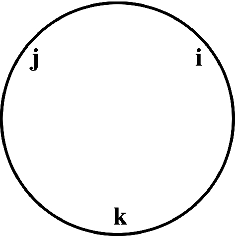
If we write the unit vectors around a circle, then reading counter clockwise gives the positive products and reading clockwise gives the negative products

Figure 25:If we write the unit vectors around a circle, then reading counter clockwise gives the positive products and reading clockwise gives the negative products

Vector Product

From the vector product definition, we can see that

i×i=j×j=k×k=0\mathbf{i}\times \mathbf{i}=\mathbf{j}\times \mathbf{j}=\mathbf{k}\times \mathbf{k}=\mathbf{0}
i×j=k,j×k=i, k×i=j\mathbf{i}\times \mathbf{j}=\mathbf{k},\mathbf{j}\times \mathbf{k}=\mathbf{i},\ \mathbf{k}\times \mathbf{i}=\mathbf{j}
j×i=k, k×j=i, i×k=j\mathbf{j}\times \mathbf{i}=-\mathbf{k},\ \mathbf{k}\times \mathbf{j}=-\mathbf{i},\ \mathbf{i}\times \mathbf{k}=-\mathbf{j}

If we write the unit vectors around a circle as shown in Figure 25, then reading counterclockwise gives the positive products and reading clockwise gives the negative products. Note that these results are for a right-handed coordinate system. We have

A×B=(Axi+Ayj+Azk)×(Bxi+Byj+Bzk)\mathbf{A}\times \mathbf{B}=(A_{x}\mathbf{i}+A_{y}\mathbf{j}+A_{z}\mathbf{k})\times (B_{x}\mathbf{i}+B_{y}\mathbf{j}+B_{z}\mathbf{k})

using the distributive law and the above relations of unit vectors we get

A×B=(AyBzAzBy)i+(AzBxAxBz)j+(AxByAyBx)k\mathbf{A}\times \mathbf{B}=(A_{y}B_{z}-A_{z}B_{y})\mathbf{i}+(A_{z}B_{x}-A_{x}B_{z})\mathbf{j}+(A_{x}B_{y}-A_{y}B_{x})\mathbf{k}

since a determinant of order 2 is defined as

a1a2b1b2=a1b2a2b1\left| \begin{array}{ll} a_{1} & a_{2}\\ b_{1} & b_{2} \end{array}\right| =a_{1}b_{2}-a_{2}b_{1}

Then, the above expression can be written as

A×B=AyAzByBziAxAzBxBzj+AxAyBxByk\mathbf{A}\times \mathbf{B}=\left| \begin{array}{ll} A_{y} & A_{z}\\ B_{y} & B_{z} \end{array}\right| \mathbf{i}-\left| \begin{array}{ll} A_{x} & A_{z}\\ B_{x} & B_{z} \end{array}\right| \mathbf{j}+\left| \begin{array}{ll} A_{x} & A_{y}\\ B_{x} & B_{y} \end{array}\right| \mathbf{k}

A determinant of order 3 is

c1c2c3a1a2a3b1b2b3=a2a3b2b3c1a1a3b1b3c2+a1a2b1b2c3\left| \begin{array}{lll} c_{1} & c_{2} & c_{3}\\ a_{1} & a_{2} & a_{3}\\ b_{1} & b_{2} & b_{3} \end{array}\right| =\left| \begin{array}{ll} a_{2} & a_{3}\\ b_{2} & b_{3} \end{array}\right| c_{1}-\left| \begin{array}{ll} a_{1} & a_{3}\\ b_{1} & b_{3} \end{array}\right| c_{2}+\left| \begin{array}{ll} a_{1} & a_{2}\\ b_{1} & b_{2} \end{array}\right| c_{3}

Hence, the cross product can be expressed as

A×B=ijkAxAyAzBxByBz=(AyBzAzBy)i+(AzBxAxBz)j+(AxByAyBx)k\mathbf{A}\times \mathbf{B}=\left| \begin{array}{lll} \mathbf{i} & \mathbf{j} & \mathbf{k}\\ A_{x} & A_{y} & A_{z}\\ B_{x} & B_{y} & B_{z} \end{array}\right| =(A_{y}B_{z}-A_{z}B_{y})\mathbf{i}+(A_{z}B_{x}-A_{x}B_{z})\mathbf{j}+(A_{x}B_{y}-A_{y}B_{x})\mathbf{k}

Note that this is not a determinant since the elements in the first row are vectors and not scalars, but it is a convenient way to represent the cross product.

Triple Product

Scalar Triple Product

The triple scalar product is a scalar quantity defined as A(B×C)\mathbf{A}\cdot (\mathbf{B}\times \mathbf{C}). This quantity can be represented by a determinant that involves the components of the vectors,

A(B×C)=AxAyAzBxByBzCxCyCz\mathbf{A}\cdot (\mathbf{B}\times \mathbf{C})=\left| \begin{array}{lll} A_{x} & A_{y} & A_{z}\\ B_{x} & B_{y} & B_{z}\\ C_{x} & C_{y} & C_{z} \end{array}\right|
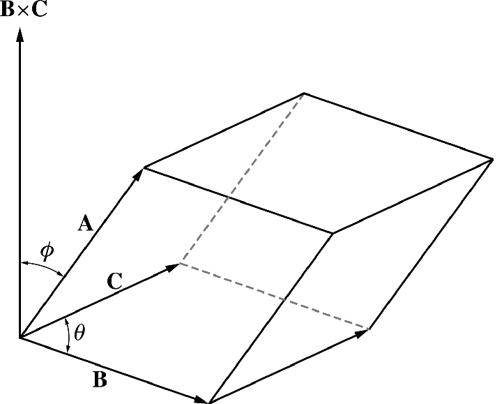
The triple scalar product is equal to the volume of a parallepiped with sides \mathbf{A}, \mathbf{B}, and \mathbf{C}

Figure 26:The triple scalar product is equal to the volume of a parallepiped with sides A,B\mathbf{A}, \mathbf{B}, and C\mathbf{C}

where A=Axi+Ayj+Azk,B=Bxi+Byj+Bzk\mathbf{A}=A_{x}\mathbf{i}+A_{y}\mathbf{j}+A_{z}\mathbf{k}, \mathbf{B}=B_{x}\mathbf{i}+B_{y}\mathbf{j}+B_{z}\mathbf{k}, and C=Cxi+Cyj+Czk.\mathbf{C}=C_{x}\mathbf{i}+C_{y}\mathbf{j}+C_{z}\mathbf{k}. Furthermore, the triple scalar product is equal to the volume of a parallepiped with sides A,B\mathbf{A}, \mathbf{B}, and C\mathbf{C} as shown in Figure 26. Because any edges can be used, the triple scalar product can be written as A(B×C)\mathbf{A} \cdot (\mathbf{B}\times \mathbf{C}) or as A(C×B)\mathbf{A}\cdot (\mathbf{C}\times \mathbf{B}) . These products are positive and negative for a right-handed coordinate system respectively. Therefore, there are 6 equal triple scalar products or 12 if you include the terms of the form (B×C)A(\mathbf{B}\times \mathbf{C})\cdot \mathbf{A} . Three of these six products are positive and the rest are negative. By expanding the determinant, you can prove that

A(B×C)=B(C×A)=C(A×B)=A(C×B)=B(A×C)=C(B×A)\mathbf{A}\cdot (\mathbf{B}\times \mathbf{C})=\mathbf{B}\cdot (\mathbf{C}\times \mathbf{A})=\mathbf{C}\cdot (\mathbf{A}\times \mathbf{B})=-\mathbf{A}\cdot (\mathbf{C}\times \mathbf{B})=-\mathbf{B}\cdot (\mathbf{A}\times \mathbf{C})=-\mathbf{C}\cdot (\mathbf{B}\times \mathbf{A})

Vector Triple Product

The triple vector product is a vector quantity defined as A×(B×C)\mathrm{A}\times (\mathrm{B}\times \mathrm{C}). You can prove by expanding this equation that

A×(B×C)=(AC)B(AB)C\mathbf{A}\times (\mathbf{B}\times \mathbf{C})=(\mathbf{A}\cdot \mathbf{C})\mathbf{B}-(\mathbf{A}\cdot \mathbf{B})\mathbf{C}

1.9 Derivatives of Vectors

If A(t)\mathbf{A}(\mathrm {t}) is a vector function of t, where t is a scalar variable such as

A(t)=Ax(t)i+Ay(t)j+Az(t)k\mathbf{A}(t)=A_{x}(t)\mathbf{i}+A_{y}(t)\mathbf{j}+A_{z}(t)\mathbf{k}

Then

dA(t)dt=dAx(t)dti+dAy(t)dtj+dAz(t)dtk\frac{d\mathbf{A}(t)}{dt}=\frac{dA_{x}(t)}{dt}\mathbf{i}+\frac{dA_{y}(t)}{dt}\mathbf{j}+\frac{dA_{z}(t)}{dt}\mathbf{k}

1.9.1 Some Rules

If A(t)\mathbf{A}(\mathrm {t}) and B(t)\mathbf{B}(\mathrm {t}) are vector functions and ϕ(t)\phi (t) is a scalar function then

ddt(ϕA)=ϕdAdt+dϕdtA\frac{d}{dt}(\phi \mathbf{A})=\phi \frac{d\mathbf{A}}{dt}+\frac{d\phi }{dt}\mathbf{A}
ddt(AB)=AdBdt+dAdtB\frac{d}{dt}(\mathbf{A}\cdot \mathbf{B})=\mathbf{A}\cdot \frac{d\mathbf{B}}{dt}+\frac{d\mathbf{A}}{dt}\cdot \mathbf{B}
ddt(A×B)=A×dBdt+dAdt×B\frac{d}{dt}(\mathbf{A}\times \mathbf{B})=\mathbf{A}\times \frac{d\mathbf{B}}{dt}+\frac{d\mathbf{A}}{dt}\times \mathbf{B}

1.9.2 Gradient, Divergence, and Curl

If A=A(x, y, z)\mathbf{A}=\mathbf{A}(x,\ y,\ z) is a vector function of x, y, and z then A(x, y, z)\mathbf{A}(x,\ y,\ z) is called a vector field. Similarly, the scalar function ϕ(x, y, z)\phi (x,\ y,\ z) is called a scalar field.

Del

The vector differential operator del is defined as

=ix+jy+kz\nabla =\mathbf{i}\frac{\partial }{\partial x}+\mathbf{j}\frac{\partial }{\partial y}+\mathbf{k}\frac{\partial }{\partial z}

Gradient

ϕ=(ix+jy+kz)ϕ=iϕx+jϕy+kϕz\nabla \phi =\bigg (\mathbf{i}\frac{\partial }{\partial x}+\mathbf{j}\frac{\partial }{\partial y}+\mathbf{k}\frac{\partial }{\partial z}\bigg )\phi =\mathbf{i}\frac{\partial \phi }{\partial x}+\mathbf{j}\frac{\partial \phi }{\partial y}+\mathbf{k}\frac{\partial \phi }{\partial z}

The vector ϕ\nabla \phi is called the gradient of ϕ\phi (written gradϕ\mathrm{grad}\,\phi).

Divergence

A=(ix+jy+kz)(Axi+Ayj+Azk)\nabla \cdot \mathbf{A}=\bigg (\mathbf{i}\frac{\partial }{\partial x}+\mathbf{j}\frac{\partial }{\partial y}+\mathbf{k}\frac{\partial }{\partial z}\bigg )\cdot (A_{x}\mathbf{i}+A_{y}\mathbf{j}+A_{z}\mathbf{k})
=Axx+Ayy+Azz=\frac{\partial A_{x}}{\partial x}+\frac{\partial A_{y}}{\partial y}+\frac{\partial A_{z}}{\partial z}

A\nabla \cdot \mathbf{A} is called the divergence of A\mathrm {A} (written div A\mathbf{A}).

Curl

×A=(ix+jy+kz)×(Axi+Ayj+Azk)\nabla \times \mathbf{A}=\bigg (\mathbf{i}\frac{\partial }{\partial x}+\mathbf{j}\frac{\partial }{\partial y}+\mathbf{k}\frac{\partial }{\partial z}\bigg )\times (A_{x}\mathbf{i}+A_{y}\mathbf{j}+A_{z}\mathbf{k})
ijkxyzAxAyAz=(AzyAyz)i+(AxzAzx)j+(AyxAxy)k\left| \begin{array}{lll} \mathbf{i} & \mathbf{j} & \mathbf{k}\\ \frac{\partial }{\partial x} & \frac{\partial }{\partial y} & \frac{\partial }{\partial z}\\ A_{x} & A_{y} & A_{z} \end{array}\right| =\bigg (\frac{\partial A_{z}}{\partial y}-\frac{\partial A_{y}}{\partial z}\bigg )\mathbf{i}+\bigg (\frac{\partial A_{x}}{\partial z}-\frac{\partial A_{z}}{\partial x}\bigg )\mathbf{j}+\bigg (\frac{\partial A_{y}}{\partial x}-\frac{\partial A_{x}}{\partial y}\bigg )\mathbf{k}

×A\nabla \times \mathbf{A} is called the curl of A\mathbf{A} (written curl A\mathbf{A}).

Some Identities

1.10 Integrals of Vectors

If A(t)=Ax(t)i+Ay(t)j+Az(t)k\mathbf{A}(t)=A_{x}(t)\mathbf{i}+A_{y}(t)\mathbf{j}+A_{z}(t)\mathbf{k}, where t is a scalar variable, the indefinite integral is defined as

A(t)dt=iAx(t)dt+jAy(t)dt+kA(t)dt\int \mathbf{A}(t)dt=\mathbf{i}\int A_{x}(t)dt+\mathbf{j}\int A_{y}(t)dt+\mathbf{k}\int A(t)dt

If A(t)=dB(t)/dt\mathbf{A}(t)=d\mathbf{B}(t)/dt, then

A(t)dt=ddt {B(t)}dt=B(t)+C\int \mathbf{A}(t)dt=\int \frac{d}{dt}\ \{\mathbf{B}(t)\} dt=\mathbf{B}(t)+\mathbf{C}

where C\mathbf{C} is an arbitrary constant vector. The definite integral between the limits t=at=a and t=bt=b is defined as

abA(t)dt=abddt {B(t)}dt=B(t)+Cab=B(b)B(a)\int _{a}^{b}\mathbf{A}(t)dt=\int _{a}^{b}\frac{d}{dt}\ \{\mathbf{B}(t)\} dt=\mathbf{B}(t)+\mathbf{C}|_{a}^{b}=\mathbf{B}(b)-\mathbf{B}(a)

1.10.1 Line Integrals

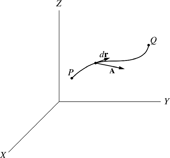
The line integral refers to an integral along a line or a curve. This curve may be open or closed. The line integral may appear in three different forms shown by cϕdr\int _{c}\phi d\mathbf{r}, cAdr\int _{c}\mathbf{A}\cdot d\mathbf{r}, and cA×dr\int _{c}\mathbf{A}\times d\mathbf{r}. The second is the most common one and it will be used throughout this book. Suppose the position vector of any point (x, y, z)(x,\ y,\ z) on the curve C\mathrm{C} (see Figure 27) that extends from P(x1, y1, z1)\mathbf{P}(x_{1},\ y_{1},\ z_{1}) at t1t_{1} to Q(x2, y2, z2)\mathbf{Q}(x_{2},\ y_{2},\ z_{2}) at t2t_{2} is given by

r(t)=x(t)i+y(t)j+z(t)k\mathbf{r}(t)=x(t)\mathbf{i}+y(t)\mathbf{j}+z(t)\mathbf{k}

where t is a scalar variable, and suppose that A=A(x, y, z)=Axi+Ayj+Azk\mathbf{A}=\mathbf{A}(x,\ y,\ z)=A_{x}\mathbf{i}+A_{y}\mathbf{j}+A_{z}\mathbf{k} is a vector field, then the line integral of A\mathbf{A} is given by

PQAdr=CAdr=C(Axdx+Aydy+Adz)\int _{P}^{Q}\mathbf{A}\cdot d\mathbf{r}=\int _{C}\mathbf{A}\cdot d\mathbf{r}=\int _{C}(A_{x}dx+A_{y}dy+Adz)

Note that Ar\mathbf{A} \cdot \mathbf{r} is the tangential component of A\mathbf{A} along C. If C\mathrm{C} is a simple closed curve (does not intersect with itself) then the line integral is written as

CAdr=C(Axdx+Aydy+Adz)\oint _{C}\mathbf{A}\cdot d\mathbf{r}=\oint _{C}(A_{x}dx+A_{y}dy+Adz)
The line integral

Figure 27:The line integral

1.10.2 Independence of Path

The line integral in general depends on the path, but sometimes it does not. Instead, it depends only on the coordinates of the end points of the curve (path) but not on the curve itself. The line integral in Eq. (110) is independent of the path, joining the points P\mathrm{P} and Q\mathrm{Q} if and only if A=ϕ\mathbf{A}=\nabla \phi, or equivalently ×A=0\nabla \times \mathbf{A}=\mathbf{0}. The value of Eq. ((110)) is then given by

PQAdr=PQdϕ=ϕ(P)ϕ(Q)=ϕ(x2, y2, z2)ϕ(x1, y1, z1)\int _{P}^{Q}\mathbf{A}\cdot d\mathbf{r}=\int _{P}^{Q}d\phi =\phi (P)-\phi (Q)=\phi (x_{2},\ y_{2},\ z_{2})-\phi (x_{1},\ y_{1},\ z_{1})

Note that ϕ(x, y, z)\phi (x,\ y,\ z) has continuous partial derivatives. Furthermore, if the line integral of A\mathbf{A} is independent of the path then the line integral of A\mathbf{A} about any closed path is equal to zero:
CAdr=0\oint _{C}\mathbf{A}\cdot d\mathbf{r}=0
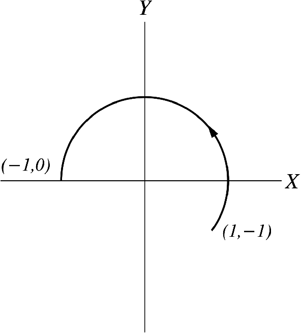
The line integral along the curve using polar coordinates

Figure 28:The line integral along the curve using polar coordinates

Problems

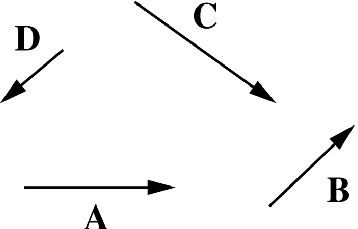
Vectors \mathbf{A}, \mathbf{B}, \mathbf{C} and \mathbf{D}

Figure 29:Vectors A,B,C\mathbf{A}, \mathbf{B}, \mathbf{C} and D\mathbf{D}