Angular momentum
Learning objectives
After this chapter, you should be able to:
use the angular-momentum commutation relations and ladder operators;
identify allowed values and measurement probabilities;
distinguish orbital and intrinsic angular momentum;
connect orbital eigenstates with spherical harmonics;
add two angular momenta using coupled and uncoupled bases;
construct the singlet and triplet states of two spin- systems;
recover the Pauli matrices of Chapter 3 as the spin- case of the general ladder construction; and
build explicit Clebsch–Gordan coefficients for coupling orbital and spin angular momentum.
9.1 The angular-momentum algebra
Chapters 1 through 4 introduced spin operationally, through Stern–Gerlach outcomes, and represented a spin- system’s observables by . That construction was built directly from the two-outcome apparatus; nothing in it referred to orbital motion. This chapter asks a more general question: what mathematical structure makes something “an angular momentum” in quantum mechanics at all? The answer is not a formula like —that expression reappears in Section 9.3, but only as one particular example—but a set of commutation relations. Anything obeying them, whatever its physical origin, inherits the entire apparatus developed below: discrete eigenvalues, ladder operators, and the role of generating rotations. Spin qualifies; so does orbital motion; so, as Section 9.4 shows, does any sum of angular momenta.
An angular momentum is, by definition, any vector operator whose Cartesian components satisfy
and cyclic permutations. This is exactly the same kind of relation already proved directly from the Pauli matrices in Chapter 3, equation (29): . What is new here is the direction of the logic. Chapter 3 started from a concrete matrix representation and derived the commutator. This chapter runs the argument in reverse: it starts from the commutator alone, treated as the defining property of “an angular momentum,” and derives everything else—the allowed eigenvalues, the ladder construction, even the existence of representations other than spin-—from that one algebraic fact. Nothing below assumes any particular matrix size in advance.
Before deriving anything from this relation, it is worth checking that it is physically plausible. Take an ordinary object—a book, a phone—and rotate it about and then about . Now reset it, and perform the same two rotations in the opposite order. The final orientations differ. Finite rotations about different axes simply do not commute, and equation (1) is the quantum statement of the corresponding infinitesimal fact: the generators of rotations about different axes cannot commute either. Section 9.3 makes this connection exact.
Its squared magnitude,
commutes with every component. This is not an additional assumption; it follows from equation (1) alone. For example,
and substituting and makes every term cancel in pairs. The same pattern holds for and by the cyclic symmetry of the algebra. Because commutes with each component, we may choose simultaneous eigenstates of and any one component—conventionally :
The allowed values are
Section 9.2 derives this restriction rather than simply asserting it. For fixed , the space has dimension . Measuring in an arbitrary state in that space returns one of the values .
Concept check 9.1
If , what values can a measurement of return?
Answer
gives , so and the possible values are .
Concept check 9.2
Does imply zero angular momentum?
Answer
No. It means only that the selected component is zero. For , the magnitude remains .
9.2 Ladder operators
Define
These are not Hermitian——so they do not represent directly measurable quantities. Their role is purely constructive: acting with or on an eigenstate produces another eigenstate with shifted by exactly one unit, which is what lets us build an entire -multiplet from a single state. The commutators
show that has shifted by one: applying to and using the commutator gives eigenvalue .
To fix the normalization—and, along the way, to see why the ladder must terminate—compute the squared norm of directly. Start by multiplying out the product term by term, exactly as you would expand for ordinary numbers:
The only difference from ordinary numbers is that and do not cancel, since and do not commute—their difference is exactly the commutator that survives in the last term. Substituting from equation (1) and then gives
Therefore
A squared norm can never be negative, so for every physically realized . Equality—a state that annihilates—occurs exactly when , not before and not after. This is the actual reason the ladder “must terminate”: it is forced by the non-negativity of a norm, the same kind of argument used throughout this book to rule out states that a formula might otherwise seem to allow. The analogous calculation with shows that annihilates a state exactly at . Together these fix both ends of the ladder, and since each application of changes by exactly one, they force the number of steps from down to —namely —to be a non-negative integer. That is precisely the statement that itself must be an integer or a half-integer. Normalizing the resulting states gives
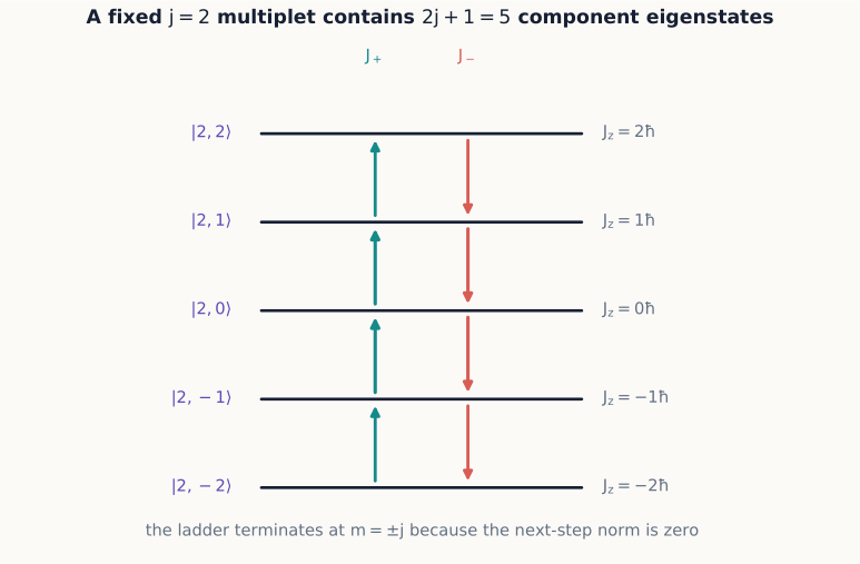
Figure 1:For fixed , the ladder operators move only among the allowed component values. Their action vanishes at , so the ladder cannot continue beyond its two physical endpoints.
The transverse components follow from
Example 9.1: a measurement
Let
The probabilities are , so and . Hence . Every term has the same , so a measurement of gives with certainty.
Example 9.2: recovering the Pauli matrices
For , the ladder relations should reproduce the Pauli-matrix spin operators of Chapter 3—after all, spin- is nothing but the representation of the same algebra. Order the two basis states as then . Equation (11) gives
and, by the same formula with the lower sign, and . In matrix form,
Combining these through , , and gives
which is exactly with the Pauli matrices defined in Chapter 3. Nothing about spin was assumed beyond : the entire matrix structure of spin- observables, including the noncommutativity that drove Chapters 2 through 4, is a special case of the abstract ladder construction.
Concept check 9.3
A calculation of for some candidate in the range comes out negative. What does this signal?
Answer
An error. The quantity equals , which is a squared norm and cannot be negative for any in the physical range; it reaches zero only at the top of the ladder, . A negative result means an arithmetic slip, not a new physical possibility.
9.3 Orbital angular momentum
For motion in space,
This is the historical origin of the name “angular momentum,” and it is one concrete realization of the abstract algebra of Section 9.1: substituting the canonical commutator (Chapter 6) into the components of shows directly that they satisfy equation (1). In spherical coordinates,
and the simultaneous eigenfunctions of and are the spherical harmonics:
For orbital motion, single-valued spatial wavefunctions require integer . The reason is direct: a wavefunction must return to the same value after , and does that only for integer , hence integer . The intrinsic spin label may also be half-integer, precisely because spin is never built from a spatial wavefunction’s dependence on in the first place—it is defined directly by the abstract algebra of Section 9.1, with no analog of “returning to the same value” to enforce. Both and obey the same operator algebra, but spin is not generated by a particle orbiting around an internal path.
A state with sharp and but indefinite is often drawn as a static cone, which makes that indefiniteness look like mere ignorance of a vector sitting still somewhere on it. The classical system that gets the geometry right is not static at all.
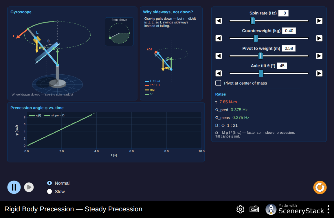
Figure 2:A spinning top under gravity: the torque stays perpendicular to , so steady precession changes the direction of the angular momentum without changing either its magnitude or its vertical component, walking the vector around the cone at fixed polar angle exactly as and remain indefinite while and stay sharp. This is the same equation of motion behind the Larmor precession of Chapter 4—a magnetic moment in a field in place of a top in gravity.
Interactive simulation: Precession
Rotation generators
A rotation through angle about is
This is the precise sense in which angular momentum “generates” rotations, foreshadowed by the noncommuting-rotations argument in Section 9.1: expanding the exponential to first order in gives , so is literally the infinitesimal generator, and composing two small rotations about different axes reproduces to leading order. For spin , and this reduces to the rotation operator of Chapter 4. Angular momentum is the generator of rotations for every quantum system.
A striking consequence follows immediately from equation (20). A full rotation about any axis gives once evaluated on an eigenbasis, and acting on this is simply the phase . For integer (hence integer ) this equals +1: a full turn returns the state unchanged, matching classical intuition. For half-integer , is also half-integer and : the state acquires an overall minus sign after one full turn and needs a second full turn to return to itself. This is not an experimental defect. It is a genuine prediction of treating spin as a angular momentum, and it has been confirmed directly with neutron interferometry.
Concept check 9.4
Orbital angular momentum requires integer . Does this mean every total angular momentum encountered in this chapter must be an integer?
Answer
No. The integer restriction in this section applies specifically to a spatial wavefunction’s single-valuedness under . Spin is not built from such a wavefunction, so it can be half-integer, and any system built by adding an odd number of half-integer spins—Sections 9.4 through 9.6—can have half-integer total as well.
9.4 Adding two angular momenta
For subsystems with and , define
Each subsystem might be two different particles’ spins, or one particle’s orbital and spin angular momenta, or the total angular momenta of two larger subsystems already built from more elementary pieces; the algebra does not care which. The uncoupled basis diagonalizes and is written . It is the natural basis for describing the two subsystems separately. The coupled basis diagonalizes and is written . It is the natural basis whenever a physical interaction or a measurement cares about the total angular momentum rather than the two parts individually—a spin–orbit coupling being the leading example, taken up in Section 9.6.
The possible totals obey the triangle rule:
In every term of a coupled-state expansion, , since . The coefficients connecting the two bases are Clebsch–Gordan coefficients. They are not arbitrary: each coupled state is built, as in the example below, by starting from the unique state of maximum and applying repeatedly, exactly as one builds any -multiplet from its top state.
A useful check on any such construction is dimension counting: the uncoupled basis has states, and the coupled basis, summing the multiplicities over the triangle-rule range of , must total the same number. This bookkeeping catches many errors before a single coefficient is computed.
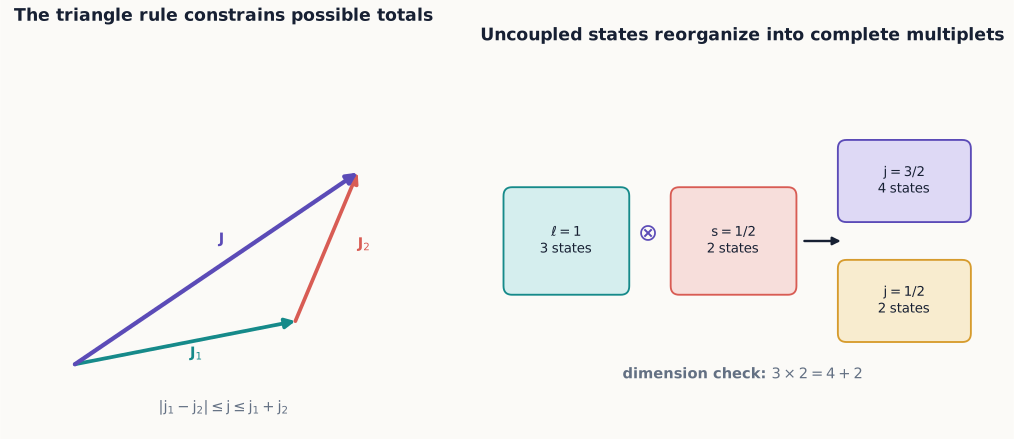
Figure 3:The triangle rule lists the allowed total magnitudes, while dimension counting checks that the coupled multiplets account for every uncoupled product state. For and , six states become a quadruplet and a doublet.
Example 9.3: coupling orbital motion and spin
Couple (a electron’s orbital angular momentum) with (its spin). The triangle rule allows and , and the dimension check confirms . Abbreviate the spin states as .
The top state is unique, since only one uncoupled combination reaches the maximum :
Lowering with and equation (11) gives on the left, while on the right and , so
Dividing both sides by the common factor isolates the ket on the left and turns the two right-hand coefficients into the Clebsch–Gordan numbers themselves:
giving
Repeating the same lowering step (Exercise 18 asks you to check this instead by lowering from the bottom of the ladder) produces
At , the uncoupled basis has two states, and ; equation (26) uses one combination, and the state orthogonal to it must be the state at the same , since and are the only totals the triangle rule allows. Choosing the conventional phase (the coefficient of the state with the larger taken positive),
Equations (26) and (28) give the Clebsch–Gordan coefficients for coupled with ; the same six coefficients reappear throughout atomic fine structure (Section 9.6) and in any -orbital spin–orbit problem.
Concept check 9.5
Why does coupling with produce one quadruplet () and one doublet (), rather than, say, two doublets with a state left over?
Answer
Dimension counting fixes it: the six uncoupled product states must reorganize into complete -multiplets. The triangle rule permits only and , and exactly accounts for all six states, with no other combination of allowed values doing so.
9.5 Two spin-one-half systems
The highest state is uniquely
Applying the total lowering operator gives
A second lowering gives . These three symmetric states form the triplet. The remaining orthogonal state is
the antisymmetric singlet.
It is worth pausing to recognize these states: equation (31) is exactly the entangled state from Chapter 5, and above is exactly . Chapter 5 introduced them as the states with the strongest possible nonclassical correlations between two separated spins, without yet having a name for why nature singles out precisely this pair of combinations. This section supplies that reason: the singlet and the triplet state are not an arbitrary choice of entangled states—they are exactly the states of definite total angular momentum, and respectively, that a rotationally symmetric interaction between two spins naturally produces and conserves. Entanglement and the addition of angular momentum turn out to be two views of the same construction for a two-spin system.
Example 9.4: measuring total spin
The product state is not an eigenstate of . Inverting the coupled-basis relations,
A total-spin measurement therefore gives or , each with probability , while is certain.
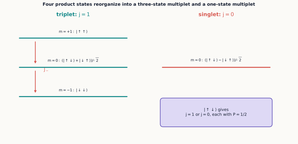
Figure 4:Coupling two spin- systems produces one symmetric triplet and one antisymmetric singlet. A product state with opposite component values has a definite but not a definite total .
Concept check 9.6
Why is the singlet unchanged by applying the same spatial rotation to both spins?
Answer
It has total , so every component of total angular momentum annihilates it. Equation (20) therefore acts as the identity on the singlet.
9.6 Coupling in atoms
An electron has orbital angular momentum and spin . Their total is , with
except that permits only —consistent with the triangle rule of Section 9.4 applied to and . Example 9.3 constructed the explicit coupled states for ; the same lowering construction works for any . A spin–orbit interaction is proportional to . Since
its energy shifts are simplest in the coupled basis: on a state built from fixed and ,
This is a general lesson: choose a basis that diagonalizes the dominant terms of the Hamiltonian and the measurement being asked about.
Example 9.5: fine-structure splitting of a level
Apply equation (35) to . For ,
while for ,
For a spin–orbit coupling of the usual (positive) sign, the energy shift is proportional to , so the level is pushed up and the level is pushed down: a single unperturbed level splits into two, with higher. This is the same splitting pattern responsible for the sodium D-line doublet, where the level’s and components acquire slightly different energies and hence emit at two closely spaced wavelengths.
Summary
Angular momentum is defined by its commutation algebra, not by any single formula; and are two realizations of the same structure.
Angular momentum has simultaneous eigenstates of and one component.
A non-negative-norm argument, not a separate postulate, forces the ladder to terminate and fixes the allowed values.
Ladder operators generate all states for a fixed , and for they exactly reproduce the Pauli matrices.
Orbital and spin angular momentum share an algebra but have different physical origins; only orbital motion is restricted to integer values.
Quantum rotations are generated by angular momentum, and half-integer states pick up a sign under a full rotation.
Coupled and uncoupled bases organize the addition of angular momenta, with Clebsch–Gordan coefficients connecting them.
Two spin-one-half systems combine into a symmetric triplet and an antisymmetric singlet; orbital and spin angular momentum combine into fine-structure multiplets with a predictable splitting pattern.
Exercises
Use equation (11) to build the matrix of for .
Calculate in the state of Example 9.1.
Show that from the component commutators.
Verify that follows from the equation.
List the allowed total values for and and verify the dimensions on both sides.
Derive all triplet states by lowering from .
Verify directly that the singlet has zero total , , and .
Find probabilities for total and in .
For and , find the eigenvalues of for both allowed values.
Explain why measuring on the singlet destroys certainty in a subsequent total-spin measurement.
Show that a rotation acts differently on integer- and half-integer- kets.
Construct projectors onto the singlet and triplet subspaces using .
Derive and use it to find the norm of , confirming it matches the lowering case of equation (11).
Using the matrices from Example 9.2, compute directly and verify it equals , consistent with .
Using the matrix for found in Exercise 1, construct and in the same basis and verify explicitly.
Verify that the four states and two states of Example 9.3 are normalized and mutually orthogonal.
A electron is prepared in . Find the probability that a measurement of returns 0.
Starting instead from in Example 9.3 and raising with , rederive and confirm it agrees with the result found by lowering from the top.
For an electron (), list the allowed values and use equation (35) to find for each.
Show that the two values found in Example 9.5 both follow from equation (35) evaluated at with .
Explain why the non-negative-norm argument behind Concept check 9.3 constrains itself, and not merely the range of available once is fixed.
A rotation about an arbitrary axis is applied to a state. State the result and compare it with the and cases.
Two electrons occupy a subshell, so . Use the triangle rule to list the allowed values of their total orbital angular momentum .
A beam of atoms with has all five outcomes equally likely. Find and .