Three-Dimensional Wave Mechanics

Three-dimensional wave mechanics¶

Learning objectives¶

After this chapter, you should be able to:

formulate normalization, probability, and Schrödinger equations in three dimensions;
separate Cartesian problems into one-dimensional factors;
interpret degeneracy in symmetric potentials;
separate central-force problems into radial and angular equations;
use radial probability densities correctly;
explain why Coulomb degeneracy exceeds what rotational symmetry alone requires; and
describe the quantum numbers and wavefunctions of hydrogen.

8.1 States in three-dimensional space¶

Chapters 1 through 7 built quantum mechanics from a small set of postulates — states as vectors, probabilities from the Born rule, unitary time evolution — first for a two-dimensional spin space and then for a particle confined to a line. None of those postulates mentioned how many dimensions space has. This chapter applies the same postulates to a particle free to move in three dimensions, which is where the theory finally meets real atoms, real scattering experiments, and real detectors. Nothing conceptually new is being added; the position label $x$ is simply replaced by the vector label $\mathbf r$ , and a single integral becomes a triple integral.

The position basis is labeled by $\mathbf r=(x,y,z)$ , with

\psi(\mathbf r)=\langle\mathbf r|\psi\rangle,\qquad \int|\psi(\mathbf r)|^2\,d^3r=1.

(1)

Quick review: the gradient and the Laplacian

Skip this box if multivariable calculus is already familiar.

In one dimension, the kinetic-energy operator involves a single second derivative, $d^2/dx^2$ . In three dimensions a wavefunction depends on all three coordinates at once, $\psi(x,y,z)$ , so “how fast $\psi$ curves” must now account for curvature along every direction, not just one. The gradient, written $\boldsymbol\nabla\psi$ , collects the three ordinary partial derivatives into a single vector,

\boldsymbol\nabla\psi= \left(\frac{\partial\psi}{\partial x}, \frac{\partial\psi}{\partial y}, \frac{\partial\psi}{\partial z}\right),

(2)

the direct three-dimensional generalization of an ordinary slope. The Laplacian, written $\nabla^2\psi$ , then adds up the second derivative along each axis separately,

\nabla^2\psi=\frac{\partial^2\psi}{\partial x^2} +\frac{\partial^2\psi}{\partial y^2} +\frac{\partial^2\psi}{\partial z^2}.

(3)

It measures total curvature: how much the value of $\psi$ at a point differs from the average of its immediate neighbors, summed over all three directions at once. Restricting $\psi$ to depend on $x$ alone recovers the one-dimensional kinetic-energy operator $-\frac{\hbar^2}{2m} \frac{d^2\psi}{dx^2}$ from Chapter 7 exactly, so nothing here is conceptually new: $\nabla^2$ is simply what $d^2/dx^2$ becomes once a wavefunction is allowed to vary in more than one direction.

For a time-independent potential,

\left[-\frac{\hbar^2}{2m}\nabla^2+V(\mathbf r)\right] \psi(\mathbf r)=E\psi(\mathbf r).

(4)

Expectation values use the volume element:

\langle A\rangle=\int \psi^*(\mathbf r)\hat A\psi(\mathbf r)\,d^3r.

(5)

The vector probability current is

\mathbf j=\frac{\hbar}{2mi} (\psi^*\boldsymbol\nabla\psi-\psi\boldsymbol\nabla\psi^*),

(6)

and obeys $\partial|\psi|^2/\partial t+\boldsymbol\nabla\cdot\mathbf j=0$ . This is the same probability current introduced in one dimension in Chapter 7, now carrying a direction as well as a magnitude: $\mathbf j$ measures how much probability flows through a small oriented patch of space per unit time, exactly as an ordinary mass or charge flux would, and the continuity equation says that probability can shift from place to place but can never be created or destroyed.

8.2 Separation in a rectangular box¶

V(x,y,z)=V_x(x)+V_y(y)+V_z(z),

(7)

a product $\psi=X(x)Y(y)Z(z)$ separates equation (4) into three one-dimensional eigenproblems, with

E=E_x+E_y+E_z.

(8)

Quick calculation: carrying out the separation¶

It is worth watching this separation happen explicitly rather than taking it on faith, since the identical technique reappears in Section 8.3 and throughout later chapters. Substituting $\psi=X(x)Y(y)Z(z)$ into equation (4) and using $V(x,y,z)=V_x(x)+V_y(y)+V_z(z)$ gives

-\frac{\hbar^2}{2m}\Big(YZ\,X''+XZ\,Y''+XY\,Z''\Big) +\big(V_x+V_y+V_z\big)XYZ=E\,XYZ.

(9)

Dividing every term by $\psi=XYZ$ separates the variables completely:

\underbrace{\left[-\frac{\hbar^2}{2m}\frac{X''}{X}+V_x(x)\right]}_{\text{function of }x\text{ alone}} +\underbrace{\left[-\frac{\hbar^2}{2m}\frac{Y''}{Y}+V_y(y)\right]}_{\text{function of }y\text{ alone}} +\underbrace{\left[-\frac{\hbar^2}{2m}\frac{Z''}{Z}+V_z(z)\right]}_{\text{function of }z\text{ alone}}=E.

(10)

The first bracket depends only on $x$ , the second only on $y$ , the third only on $z$ —yet their sum is the single constant $E$ , the same number regardless of $x$ , $y$ , or $z$ . The only way three functions of independent variables can add up to one fixed constant for every choice of $x$ , $y$ , and $z$ is if each bracket is separately equal to its own constant:

-\frac{\hbar^2}{2m}\frac{d^2X}{dx^2}+V_x(x)X=E_xX,

(11)

and likewise for $Y$ with constant $E_y$ and $Z$ with constant $E_z$ , where $E=E_x+E_y+E_z$ . One three-dimensional problem has become three ordinary one-dimensional eigenvalue problems, each of exactly the form already solved in Chapter 7.

For an infinite rectangular box with sides $L_x,L_y,L_z$ ,

\psi_{n_xn_yn_z} =\sqrt{\frac{8}{L_xL_yL_z}} \sin\frac{n_x\pi x}{L_x} \sin\frac{n_y\pi y}{L_y} \sin\frac{n_z\pi z}{L_z},

(12)

E_{n_xn_yn_z} =\frac{\pi^2\hbar^2}{2m} \left(\frac{n_x^2}{L_x^2} +\frac{n_y^2}{L_y^2} +\frac{n_z^2}{L_z^2}\right).

(13)

In a cube, permutations such as $(1,1,2)$ , $(1,2,1)$ , and $(2,1,1)$ have the same energy. This degeneracy reflects the box’s symmetry. Changing one side length breaks the symmetry and usually splits those energies.

Concept check 8.1¶

In a cubic box, are $(1,1,2)$ and $(1,2,1)$ the same state?

The cube’s degeneracy comes from a geometric symmetry: permuting $x$ , $y$ , and $z$ leaves the Hamiltonian unchanged, so states related by that permutation must share an energy. Section 8.5 will meet a second kind of degeneracy in the hydrogen atom that cannot be explained this way. Keeping these two origins distinct now will make the hydrogen case less mysterious later.

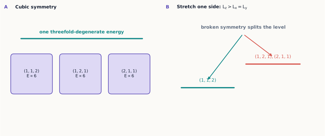
Figure 1:Permuting the quantum numbers of a cubic box does not change the energy. Stretching one side distinguishes that direction, partially lifting the degeneracy and exposing its geometric origin.

8.3 Central potentials and spherical coordinates¶

Quick review: spherical coordinates

Skip this box if $(r,\theta,\phi)$ is already a familiar coordinate system.

Ordinary Cartesian coordinates $(x,y,z)$ locate a point by three signed distances along fixed axes. Spherical coordinates instead locate the same point using one distance and two angles: $r\ge0$ is the distance from the origin, $\theta\in[0,\pi]$ is the polar angle measured down from the $+z$ axis, and $\phi\in[0,2\pi)$ is the azimuthal angle measured around the $z$ axis—the same way longitude is measured around the Earth, with $\theta$ playing the role of colatitude. The conversion to Cartesian coordinates is

x=r\sin\theta\cos\phi,\qquad y=r\sin\theta\sin\phi,\qquad z=r\cos\theta.

(14)

This system earns its keep whenever the physics singles out one special point, the origin, and treats every direction away from it on equal footing—exactly the situation for a central potential $V(r)$ , which depends on distance from the origin alone and not on direction at all. Rewriting the Laplacian in these coordinates is what allows a problem with spherical symmetry to be split into a radial equation depending on $r$ alone, plus angular equations depending only on $\theta$ and $\phi$ —precisely the split carried out in equation (15) next, by the same separation-of-variables logic just used for the rectangular box.

When $V(\mathbf r)=V(r)$ , spherical coordinates respect the rotational symmetry. Write

\psi(r,\theta,\phi)=R(r)Y(\theta,\phi).

(15)

Separation produces angular eigenfunctions $Y_\ell^m$ , introduced fully in Chapter 9, and a radial equation.

The centrifugal term below is not an extra assumption; it is what remains of the Laplacian’s angular part. In spherical coordinates the Laplacian splits into a radial piece and an angular piece,

\nabla^2=\frac1{r^2}\frac{\partial}{\partial r} \left(r^2\frac{\partial}{\partial r}\right) -\frac{\hat L^2}{\hbar^2r^2},

(16)

where $\hat L^2$ is built entirely from angular derivatives — the same orbital-angular-momentum operator whose eigenstates and eigenvalues Chapter 9 derives from first principles. Its eigenfunctions are exactly the spherical harmonics,

\hat L^2Y_\ell^m=\hbar^2\ell(\ell+1)Y_\ell^m,

(17)

so substituting $\psi=R(r)Y_\ell^m(\theta,\phi)$ into (4) replaces $\hat L^2$ by its eigenvalue and leaves an ordinary differential equation in $r$ alone, with $\ell(\ell+1)$ appearing as a fixed number rather than an operator. Writing $u(r)=rR(r)$ removes the first-derivative term from that equation and gives the compact form used throughout this chapter:

-\frac{\hbar^2}{2m}\frac{d^2u}{dr^2} +\left[V(r)+\frac{\hbar^2\ell(\ell+1)}{2mr^2}\right]u =Eu.

(18)

The term

V_{\mathrm{cent}}(r)=\frac{\hbar^2\ell(\ell+1)}{2mr^2}

(19)

is the centrifugal contribution. It repels states with $\ell>0$ from the origin even when the physical potential is attractive.

The spherical volume element is $d^3r=r^2\sin\theta\,dr\,d\theta\,d\phi$ . If the spherical harmonic is normalized, the probability of finding the particle between $r$ and $r+dr$ is

P(r)\,dr=r^2|R(r)|^2dr=|u(r)|^2dr.

(20)

The radial probability is not $|R(r)|^2$ alone. The factor $r^2$ counts the growing volume of spherical shells.

Example 8.1: where is a $1s$ electron most likely?¶

For hydrogen,

\psi_{100}(r)=\frac{1}{\sqrt{\pi a_0^3}}e^{-r/a_0}.

(21)

The spatial density is largest at $r=0$ , but the radial density is

P(r)=\frac{4r^2}{a_0^3}e^{-2r/a_0}.

(22)

Differentiating with the product rule,

\frac{dP}{dr}=\frac{4}{a_0^3}\left(2re^{-2r/a_0} -\frac{2r^2}{a_0}e^{-2r/a_0}\right) =\frac{8r}{a_0^3}e^{-2r/a_0}\left(1-\frac{r}{a_0}\right),

(23)

which vanishes at $r=0$ (a minimum, since $P(0)=0$ there) and at $r=a_0$ . The second root is the most probable radius, matching the length scale already built into the wavefunction itself. “Most likely point” and “most likely radius” answer different questions because their volume elements differ. Example 8.2 revisits this distinction for a state with nonzero $\ell$ , where the growing shell volume and the decaying exponential compete at a larger radius.

Concept check 8.2¶

Why can $|\psi(0)|^2$ be largest at the origin while the probability of finding the particle at exactly the origin is zero?

8.4 The hydrogen atom¶

For an electron and proton, the center-of-mass motion separates from their relative coordinate. The relative particle has reduced mass

\mu=\frac{m_em_p}{m_e+m_p}

(24)

Quick review: why a reduced mass appears

Skip this box if the two-body-to-one-body reduction is already familiar from classical mechanics.

The hydrogen atom is really a two-body problem: an electron and a proton, each free to move, pulling on each other. Attacking the Schrödinger equation directly for two independent three-dimensional positions would mean six coordinates at once. Exactly as in classical mechanics, this splits cleanly into two separate and much simpler problems: the motion of the center of mass, which drifts freely like a single particle of total mass $m_e+m_p$ and carries no information about the atom’s internal structure, and the motion of the relative coordinate $\mathbf r=\mathbf r_e-\mathbf r_p$ , which behaves exactly like one fictitious particle orbiting a fixed center— provided that fictitious particle is assigned the reduced mass $\mu=m_em_p/(m_e+m_p)$ rather than either individual mass. Because $m_p\approx1836\,m_e$ , $\mu$ turns out extremely close to $m_e$ itself, close enough that using $m_e$ in its place is an excellent approximation for most purposes—though not for the highest-precision spectroscopy, and not when comparing hydrogen to deuterium, where the small difference in $\mu$ is exactly the quantity being measured.

and Coulomb potential

V(r)=-\frac{e^2}{4\pi\epsilon_0r}.

(25)

Normalizable solutions are labeled by

n=1,2,\ldots,\qquad \ell=0,1,\ldots,n-1,\qquad m=-\ell,\ldots,\ell.

(26)

Ignoring spin and small corrections, the energy depends only on $n$ :

E_n=-\frac{\mu e^4} {2(4\pi\epsilon_0)^2\hbar^2}\frac1{n^2} =-\frac{13.6\ \mathrm{eV}}{n^2}

(27)

when the reduced-mass correction is rounded to the usual value. The wavefunction factors as

\psi_{n\ell m}(r,\theta,\phi) =R_{n\ell}(r)Y_\ell^m(\theta,\phi).

(28)

The principal quantum number $n$ sets the energy in the ideal Coulomb problem; $\ell$ sets the orbital angular-momentum magnitude; and $m$ sets its component along the chosen $z$ axis.

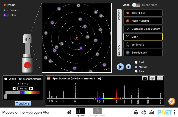
Screenshot of the Models of the Hydrogen Atom simulation — Figure 2:Compare the Bohr, de Broglie, and Schrödinger pictures of hydrogen side by side, and fire simulated photons at each model to see which one’s predictions actually match the observed emission and absorption spectrum.
Interactive simulation: Models of the Hydrogen Atom

Concept check 8.3¶

Does the quantum number $m$ specify a three-dimensional orbital plane?

Nodes and scales¶

The angular function has $\ell-|m|$ angular nodes in polar angle, together with azimuthal phase structure. The radial function has $n-\ell-1$ radial nodes. The total number of radial plus angular nodes is $n-1$ .

The natural length is the Bohr radius

a_0=\frac{4\pi\epsilon_0\hbar^2}{\mu e^2}.

(29)

Hydrogen orbitals are stationary probability amplitudes, not classical paths traced by an electron. Names such as $s,p,d$ refer to $\ell=0,1,2$ , not to little planetary orbits.

A checkable energy split: the Virial theorem

For any power-law potential $V(r)\propto r^k$ , the Virial theorem relates the average kinetic and potential energies in a bound stationary state: $2\langle T\rangle=k\langle V\rangle$ . The Coulomb potential has $k=-1$ , so $2\langle T\rangle=-\langle V\rangle$ . Combined with $E=\langle T\rangle+\langle V\rangle$ , this fixes both pieces separately:

\langle T\rangle=-E_n,\qquad\langle V\rangle=2E_n.

(30)

For $n=1$ , $E_1=-13.6\ \mathrm{eV}$ gives $\langle T\rangle=+13.6\ \mathrm{eV}$ and $\langle V\rangle=-27.2\ \mathrm{eV}$ — a compact, numerically checkable statement about how a hydrogen electron’s energy divides between motion and attraction, without integrating the kinetic and potential operators separately.

Example 8.2: size and shape of a $2p$ orbital¶

The normalized $n=2,\ell=1$ radial function is

R_{21}(r)=\frac{1}{2\sqrt6}\,a_0^{-3/2}\,\frac{r}{a_0}\,e^{-r/(2a_0)}.

(31)

Its radial probability density is

P(r)=r^2R_{21}^2(r)=\frac{1}{24a_0^5}\,r^4e^{-r/a_0}.

(32)

Differentiating with the product rule, treating $1/(24a_0^5)$ as a constant prefactor,

\frac{dP}{dr}=\frac{1}{24a_0^5} \left(4r^3e^{-r/a_0}-\frac{r^4}{a_0}e^{-r/a_0}\right) =\frac{e^{-r/a_0}}{24a_0^5}\left(4r^3-\frac{r^4}{a_0}\right).

(33)

Setting $dP/dr=0$ gives $4r^3-r^4/a_0=0$ (the exponential factor is never zero, so only the polynomial part can vanish), so the most probable radius is $r_{\max}=4a_0=n^2a_0$ — the same radius Bohr’s original circular-orbit picture assigns to $n=2$ , even though the orbital has no orbit.

Quick review: the integral

\int_0^\infty x^ne^{-x/a}\,dx=n!\,a^{n+1}

This integral—a rescaled Gamma-function integral—appears every time a hydrogen radial probability, always a polynomial in $r$ times $e^{-r/a_0}$ , is integrated to get a normalization constant or a mean value, so it is worth keeping on hand as a standing tool rather than re-deriving it by repeated integration by parts each time it is needed. A quick check at small $n$ builds confidence in it: for $n=0$ , $\int_0^\infty e^{-x/a}\,dx=a=0!\,a^1$ ; integrating once by parts for $n=1$ gives $\int_0^\infty xe^{-x/a}\,dx=a^2=1!\,a^2$ . Each additional power of $x$ contributes one more integration by parts, and hence one more factor of $a$ together with one more factor in the falling product that becomes $n!$ —exactly the pattern the general formula packages into one closed form.

The mean radius, by contrast, is

\langle r\rangle=\int_0^\infty rP(r)\,dr =\frac{1}{24a_0^5}\int_0^\infty r^5e^{-r/a_0}\,dr =\frac{5!\,a_0^6}{24a_0^5}=5a_0,

(34)

somewhat larger than $r_{\max}$ because the exponential tail pulls the average outward. The same pattern held for the $1s$ state in Example 8.1 ( $r_{\max}=a_0$ , $\langle r\rangle=\tfrac32a_0$ , Exercise 6): a skewed distribution’s most probable value and its mean are different numbers answering different questions, and neither should be read as “the orbital’s radius” without saying which one is meant. In general,

\langle r\rangle_{n\ell}=\frac{a_0}{2}\left[3n^2-\ell(\ell+1)\right],

(35)

which reproduces both results above and lets Exercises 15–16 extend the comparison to other orbitals without repeating the integral from scratch.

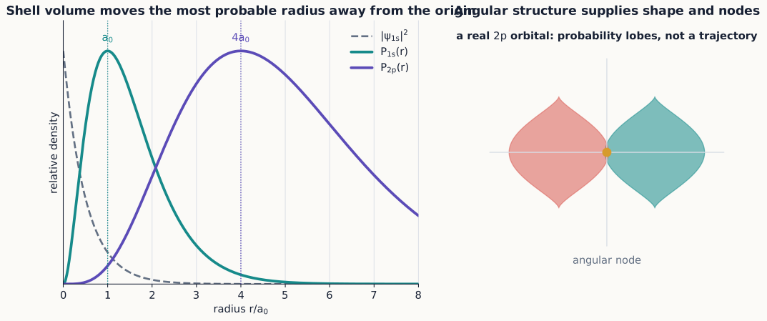
Curves compare the hydrogen 1s point density with 1s and 2p radial probability densities, whose peaks occur at one and four Bohr radii. A two-lobed real 2p orbital shows opposite phases separated by an angular node. — Figure 3:The shell-volume factor moves radial-probability peaks away from the point where the spatial density is largest. Angular factors add lobes, phases, and nodes; none of these structures represents a classical electron orbit.

Concept check 8.4¶

For the $2p$ orbital of Example 8.2, why is $\langle r\rangle=5a_0$ larger than the most probable radius $r_{\max}=4a_0$ ?

8.5 Degeneracy and symmetry¶

For fixed $n$ , the allowed orbital states number

\sum_{\ell=0}^{n-1}(2\ell+1)=n^2.

(36)

This is worth checking directly for the first few values of $n$ before trusting it in general. For $n=1$ , only $\ell=0$ contributes: $1=1^2$ . For $n=2$ , $\ell=0$ and $\ell=1$ contribute $1+3=4=2^2$ . For $n=3$ , $\ell=0,1,2$ contribute $1+3+5=9=3^2$ . The pattern is just the familiar fact that the first $n$ odd numbers always sum to $n^2$ , now dressed up in the $(2\ell+1)$ -fold degeneracy that rotational symmetry assigns to each value of $\ell$ . Including two spin states doubles this count. The Coulomb degeneracy is larger than rotational symmetry alone requires: states with different $\ell$ also share the same energy. This is a genuinely different phenomenon from the box degeneracy of Section 8.2. Rotational symmetry by itself only guarantees the $(2\ell+1)$ -fold degeneracy in $m$ at fixed $\ell$ ; it says nothing about why the $2s$ and $2p$ levels should coincide. The extra, exact $1/r$ dependence of the Coulomb potential hides a larger symmetry beyond ordinary rotations — associated with a conserved Runge–Lenz vector and often described as an $\mathrm{SO}(4)$ symmetry of the classical and quantum Kepler problem. Working out that symmetry is beyond this book’s scope, but it is worth knowing by name: “accidental” degeneracy in hydrogen is not an accident at all, and it is fragile for exactly that reason. Relativistic corrections, spin–orbit coupling, external electric or magnetic fields, and finite nuclear effects break the exact $1/r$ form and lift parts of this degeneracy.

Concept check 8.5¶

Is the degeneracy between the cubic-box states $(1,1,2)$ and $(2,1,1)$ the same kind of phenomenon as the degeneracy between hydrogen’s $2s$ and $2p$ states?

Degenerate states may be combined into other stationary states of the same energy. For example, real linear combinations of $m=\pm1$ orbitals can be oriented along different spatial axes. Choosing a basis within a degenerate subspace is often guided by the additional interaction or measurement being considered.

8.6 Spectra and selection ideas¶

If an atom changes from energy $E_i$ to $E_f$ while emitting or absorbing one photon, energy conservation gives

\hbar\omega=|E_f-E_i|.

(37)

Not every energy difference necessarily appears with equal strength. The coupling operator and the angular symmetries determine transition amplitudes. For electric-dipole coupling, the most common orbital rules are $\Delta\ell=\pm1$ and $\Delta m=0,\pm1$ . These are not extra prohibitions placed on energy conservation; they identify matrix elements that vanish by symmetry.

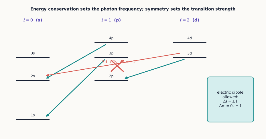
Hydrogen s, p, and d sublevels are arranged by energy. Arrows connect electric-dipole-allowed transitions that change orbital angular momentum by one, while a 3d to 2s transition changing it by two is crossed out. — Figure 4:Energy differences determine possible photon frequencies, while symmetry determines which transitions have nonzero electric-dipole amplitudes. An energetically possible line may therefore be absent or extremely weak.

Why $\Delta\ell=\pm1$ : a parity argument¶

Quick review: even and odd functions, and parity

Skip this box if “parity” already means something concrete to you.

A function $f(x)$ is called even if $f(-x)=f(x)$ —flipping the sign of its argument leaves it unchanged, like $\cos x$ or $x^2$ —and odd if $f(-x)=-f(x)$ , like $\sin x$ or $x$ itself. The key fact used repeatedly below concerns integrals: the integral of an odd function over a range symmetric about the origin, such as $\int_{-a}^{a}f(x)\,dx$ with $f$ odd, is always exactly zero, since whatever the function contributes on the positive side is exactly canceled by its mirror image on the negative side. An even function has no such automatic cancellation.

Parity is this same even/odd idea promoted to three dimensions, where “flipping the sign of the argument” means reflecting every point through the origin, $\mathbf r\to-\mathbf r$ . A three-dimensional function has even parity if it is unchanged by this reflection and odd parity if it flips sign, and the identical cancellation argument applies: an integral over all of space of a function with overall odd parity vanishes automatically, with no need to know any further details of the function. This is exactly the tool the argument below applies to the electric-dipole matrix element.

The rate for an electric-dipole transition is controlled by a matrix element of the position operator, $\langle n'\ell'm'|\mathbf r|n\ell m\rangle$ . Under spatial inversion $\mathbf r\to-\mathbf r$ , a spherical harmonic picks up a definite sign, $Y_\ell^m\to(-1)^\ell Y_\ell^m$ , while $\mathbf r$ itself is odd. The full integrand therefore transforms with an overall factor $(-1)^{\ell'}(-1)(-1)^\ell=(-1)^{\ell+\ell'+1}$ . Since the integral runs over all directions symmetrically, it can be nonzero only if this factor is +1, which requires $\ell+\ell'$ to be odd. This already forbids $\Delta\ell=0,\pm2,\ldots$ on symmetry grounds alone, independent of any detailed radial integral.

Parity alone would still allow $\Delta\ell=\pm1,\pm3,\ldots$ . The tighter rule comes from angular momentum: the dipole operator behaves like an object carrying one unit of angular momentum, and Chapter 9 shows that combining angular momentum $\ell$ with one added unit can only produce a total in the range $|\ell-1|$ to $\ell+1$ . Intersecting that with the odd- $\ell+\ell'$ requirement leaves exactly $\Delta\ell=\pm1$ . The $\Delta m=0,\pm1$ rule has an analogous origin: the three dipole components behave as objects with definite angular-momentum projection $q=0,\pm1$ along $z$ , and the $\phi$ integral vanishes unless $m'=m+q$ .

Concept check 8.6¶

A student argues that a $3d\to2s$ transition should be electric-dipole allowed because energy is released and $\Delta n\ne0$ . Is the student correct?

Summary¶

Three-dimensional wave mechanics uses the Laplacian and the physical volume element.
Separable potentials reduce to lower-dimensional eigenproblems.
Degeneracy reflects symmetry and allows many eigenstates to share one energy.
Central potentials separate into radial functions and spherical harmonics.
Radial probabilities include a factor $r^2$ ; the most probable radius and the mean radius generally differ.
The Coulomb potential’s centrifugal term traces back to the eigenvalue of $\hat L^2$ inside the Laplacian.
The Virial theorem fixes $\langle T\rangle=-E_n$ and $\langle V\rangle=2E_n$ for hydrogen.
Hydrogen states are labeled by $n,\ell,m$ , with ideal Coulomb energies depending only on $n$ ; this extra degeneracy reflects a dynamical symmetry beyond ordinary rotations, distinct from the geometric degeneracy of a symmetric box.
Electric-dipole selection rules ( $\Delta\ell=\pm1$ , $\Delta m=0,\pm1$ ) follow from parity and angular-momentum addition, not from energy conservation.

Exercises¶

Normalize the rectangular-box state in equation (12).
List the degeneracies of the first four distinct energy values in a cubic box.
Show how a small change $L_z\ne L_x=L_y$ splits the $(1,1,2)$ family.
Derive equation (18) from the spherical-coordinate Laplacian, using $u=rR$ .
Normalize the hydrogen $1s$ radial probability and verify that its maximum occurs at $a_0$ .
Calculate $\langle r\rangle$ for the $1s$ state.
List all $(\ell,m)$ pairs for $n=3$ and verify that there are nine orbital states.
Count the radial and angular nodes for $3s$ , $3p$ , and $3d$ states.
Find the wavelength of a photon emitted in the ideal hydrogen transition $n=3$ to $n=2$ .
Explain why an arbitrary superposition inside one degenerate energy subspace is stationary up to an overall phase.
Give the electric-dipole-allowed possibilities for $(\ell,m)=(1,0)$ .
Compare position density, radial density, and probability in a thin spherical shell; state the units of each.
Substitute $\psi=R(r)Y_\ell^m(\theta,\phi)$ into equation (4), use equation (16) and $\hat L^2Y_\ell^m=\hbar^2\ell(\ell+1)Y_\ell^m$ , and reduce the result to equation (18) with $u=rR$ .
Verify directly that $R_{21}(r)$ in Example 8.2 satisfies $\int_0^\infty R_{21}^2(r)\,r^2\,dr=1$ .
The normalized $2s$ radial function is $R_{20}(r)=\frac{1}{2\sqrt2}a_0^{-3/2}\left(2-\dfrac{r}{a_0}\right) e^{-r/(2a_0)}$ . Find its radial node, and use equation (35) to find $\langle r\rangle$ for $2s$ . Explain why it differs from the $2p$ result of Example 8.2 even though both belong to $n=2$ .
Use equation (30) to predict $\langle T\rangle$ and $\langle V\rangle$ for $n=2$ and $n=3$ .
Using $\langle1/r\rangle_{1s}=1/a_0$ , compute $\langle V\rangle=-\dfrac{e^2}{4\pi\epsilon_0}\langle1/r\rangle$ for the $1s$ state directly and confirm it equals $2E_1$ , as required by equation (30).
Using the parity argument of Section 8.6, decide which of these transitions are electric-dipole allowed: $3d\to2p$ , $3d\to2s$ , $3p\to1s$ , $3s\to2s$ .
Explain, using the angular-momentum addition idea previewed in Section 8.6, why $\Delta\ell=\pm3$ is forbidden even though $\ell+\ell'$ is odd for such a transition.
A rectangular box has $L_x=L$ , $L_y=2L$ , $L_z=3L$ . List its five lowest distinct energies in units of $\pi^2\hbar^2/(2mL^2)$ and state whether any of them are degenerate.
A weak external electric field is turned on in a hydrogen atom (the Stark effect). Using the distinction drawn in Section 8.5, explain qualitatively why this field can split the four degenerate $n=2$ levels even though it is not a rotation. (Chapter 10 develops the quantitative tool for this calculation.)
Using $R_{20}$ from Exercise 15, find the most probable radius for the $2s$ state. Does it equal $n^2a_0=4a_0$ as it did for $2p$ in Example 8.2? What feature of the $2p$ state made $r_{\max}=n^2a_0$ work there?
Considering only decays to $n=2$ , list every electric-dipole-allowed final state reachable from $3d,\ m=0$ and from $3p,\ m=0$ , applying both the $\Delta\ell=\pm1$ and $\Delta m=0,\pm1$ rules.
Explain in your own words why the phrase “hydrogen’s degeneracy is accidental” is misleading, using the vocabulary introduced in Section 8.5.

Three-Dimensional Wave Mechanics