Modern quantum applications
Learning objectives
After this chapter, you should be able to:
represent quantum logic operations as unitary gates;
explain no-cloning, teleportation, and superdense coding;
distinguish decoherence from measurement uncertainty;
state the purpose of quantum error correction;
connect two-state dynamics to clocks, magnetic resonance, and sensing;
illustrate how phase kickback lets a quantum algorithm answer a global question about a function with fewer queries than any classical algorithm (Deutsch’s algorithm); and
evaluate quantum-technology claims in terms of states, transformations, measurements, and resources.
12.1 From spin states to qubits
A qubit is any controlled two-state quantum system:
The physical realization might use spin, atomic energy levels, photon polarization, superconducting circuits, or another pair of states. Different hardware has different control and noise, but the same two-dimensional formalism applies.
Common one-qubit gates include
They are unitary transformations, not measurements. The gate exchanges and ; changes a relative sign; Hadamard converts between and bases; and adds a quarter-cycle phase.
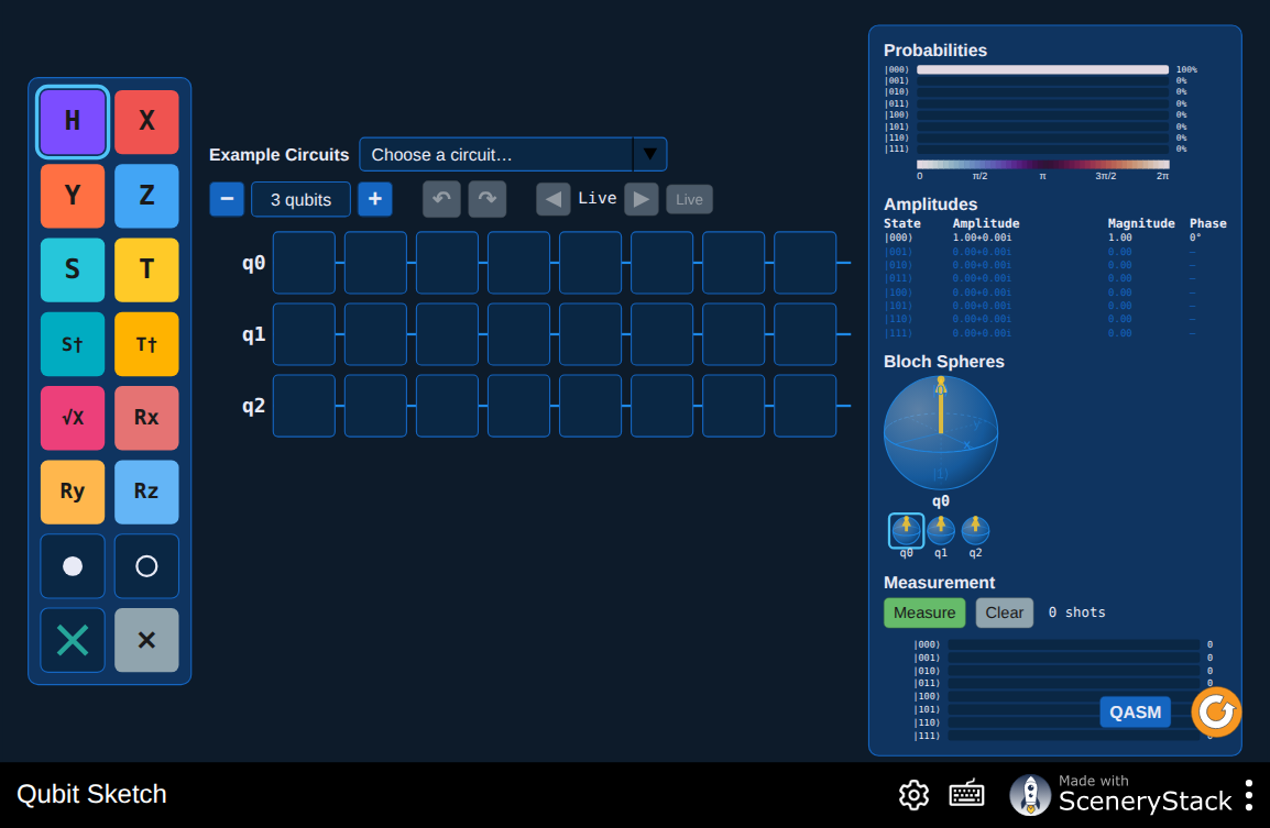
Figure 1:Drag , , , and gates onto a single qubit and watch its Bloch sphere and amplitudes update after each one—the same circuit builder used in Chapter 5 to entangle two qubits, now applied one gate at a time to a single qubit’s state.
Interactive simulation: Qubit Sketch
12.2 Circuits and quantum information
A circuit diagram is read in time order. Gates compose as matrix products, and measurement converts final amplitudes into classical records. A useful calculation always specifies the input, applies gates in order, and projects in the stated measurement basis.
The no-cloning theorem
Suppose one unitary could copy every unknown state using a single fixed, fresh ancilla :
Unitary evolution preserves inner products, so the overlap can be evaluated two ways. Using gives one value; substituting the cloning hypothesis gives another:
Both expressions describe the same quantity, so writing turns equation (4) into , or . Only or solves this: a single fixed can reproduce the cloning relation for a pair of states that are already orthogonal or already identical up to normalization, never for a generic unknown pair with . A device can copy a known orthogonal basis, such as , but no physical operation perfectly clones an arbitrary unknown qubit.
No-cloning is not a technological inconvenience. It follows from linearity alone and protects the distinction between quantum information and an unknown classical description: if an unknown qubit could always be silently duplicated, no protocol whose security or correctness depends on that impossibility could work. It is also why the teleportation protocol below must destroy the sender’s local access to as the price of reconstructing it elsewhere—transmitting quantum information can never mean copying it.
Concept check 12.1
Why can a controlled-NOT gate copy and without violating no-cloning?
Answer
No-cloning forbids copying every unknown state. CNOT copies the selected orthogonal basis, but an input superposition produces entanglement rather than two independent copies.
12.3 Teleportation
Quantum teleportation transfers an unknown qubit state using shared entanglement and two classical bits. Let qubit 1 contain , while qubits 2 and 3 share . Reexpressing the three-qubit state in the Bell basis of qubits 1 and 2 gives
A Bell-basis measurement on 1 and 2 gives one of four random outcomes. Sending its two-bit label allows the holder of qubit 3 to apply the corresponding correction and recover .
The original qubit is not copied: the measurement destroys its prior local state, consistent with no-cloning. The receiver cannot recover before the classical message arrives, so teleportation does not send information faster than light.
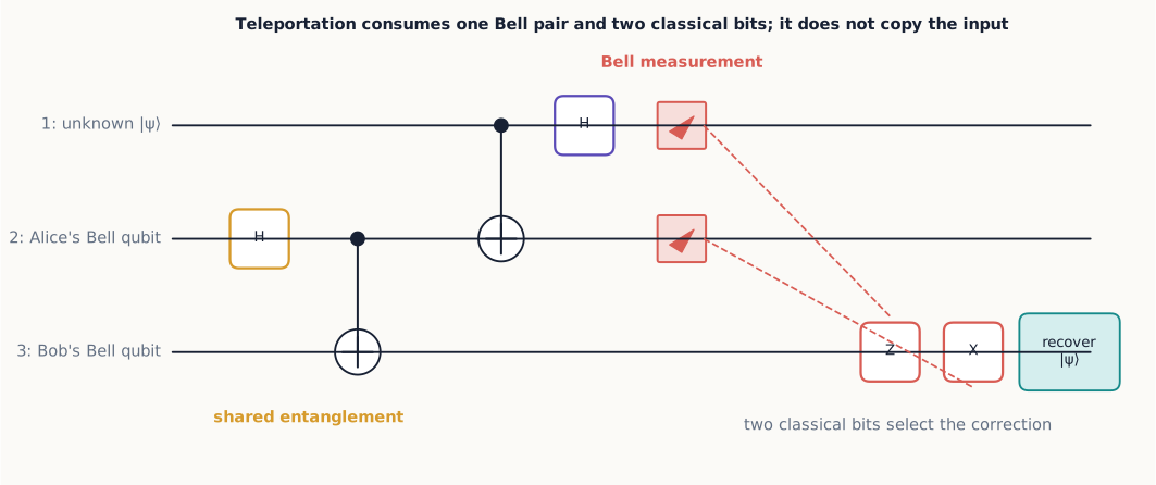
Figure 2:Teleportation relocates a preparation by combining a shared Bell pair with two classical bits. The Bell measurement removes the sender’s local copy, and the receiver obtains the state only after the outcome-dependent correction.
Concept check 12.2
Does teleportation eliminate the need to transmit information?
Answer
No. It consumes shared entanglement and requires two ordinary classical bits. Without them, the receiver’s local state contains no accessible copy of the unknown input.
Example 12.1: a concrete correction
Let , so and in equation (5). Suppose the Bell measurement on qubits 1 and 2 returns the outcome . Immediately afterward—before any correction is applied—qubit 3 is left in
This is not , and by itself it carries no information about which of the four outcomes occurred at the sender. The two classical bits naming tell the receiver to undo . Because and do not commute, the order of the correction matters: applying and then ,
exactly recovers the original state. Applying the same two corrections in the opposite order returns instead—physically indistinguishable from , since an overall phase carries no observable consequence (Chapter 2), but not identical as a vector, so a careful statement of the protocol fixes one convention. In the vocabulary that will organize the rest of this chapter (Section 12.9), the preparation reconstructed at qubit 3 depends on both the shared entangled resource and the classical record of the measurement at the sender; neither the entanglement alone nor the two bits alone would be evidence of a transferred qubit.
Concept check 12.3
In Example 12.1, does the sender end up holding a usable copy of after the Bell measurement?
Answer
No. The Bell measurement projects qubits 1 and 2 into an entangled two-qubit outcome state, leaving qubit 1 with no local state that recovers . If the sender also retained a usable copy while qubit 3 ended up with , two independent copies of an unknown state would exist, contradicting no-cloning.
Superdense coding
The resource accounting can be reversed. If two parties share a Bell pair, one party can apply one of to encode two classical bits in the joint Bell state, then transmit one qubit. A Bell measurement recovers the two-bit message. The protocol consumes prior entanglement plus one transmitted qubit; it does not encode arbitrarily many bits in one unassisted two-state system.
12.4 Decoherence and open systems
Useful quantum behavior depends on controlled relative phases. Unmonitored degrees of freedom can become correlated with a system:
If the environment states become distinguishable and are not observed, tracing them out suppresses the qubit’s off-diagonal density-matrix elements. This is decoherence. It explains the loss of interference in an open subsystem without requiring a person to inspect the environment.
Two common time scales are:
, energy relaxation toward thermal populations; and
, loss of phase coherence.
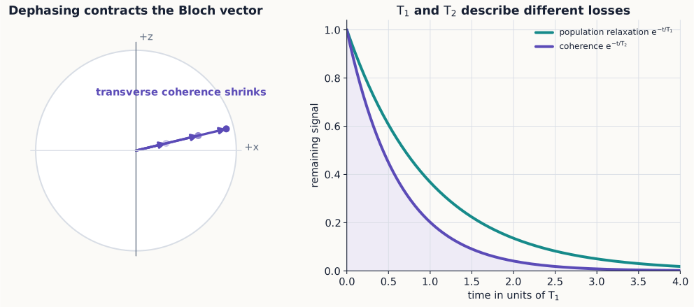
Figure 3:Decoherence turns a sharp Bloch vector into a shorter mixed-state vector. tracks population relaxation, while tracks transverse phase coherence; a device must characterize both rather than quote one lifetime.
Typically , and additional low-frequency noise can make it much shorter. Gate times must be small compared with relevant coherence times, but that ratio alone does not fully characterize correlated errors, leakage, or measurement faults.
Example 12.2: comparing a gate time with coherence times
A two-qubit gate takes on a qubit with and . Modeling the decay as simple exponentials and ,
A single gate loses under half a percent of population and about two-thirds of a percent of coherence—consistent with the qualitative requirement above. But small per-gate losses compound over a circuit: after such gates run back to back, the coherence factor is roughly , which would destroy essentially all interference long before is reached in absolute time. A short ratio is necessary for one gate to be useful, but a circuit of any depth needs many gates, which is exactly why quantum error correction—not coherence time by itself—is needed to run long computations. In the language of Section 12.9, decoherence is a transformation imposed by an uncontrolled environment rather than a chosen one, and its accumulated effect over a circuit is part of the evidence that must be checked against any performance claim.
12.5 Quantum error correction
Classical repetition cannot be applied by first cloning an unknown qubit. Quantum error correction instead encodes one logical state into an entangled subspace of several physical qubits. Carefully chosen syndrome measurements reveal which error occurred without revealing the logical amplitudes .
For example, the three-qubit repetition code maps
Parity checks can locate one bit-flip error, after which a correction restores the encoded state. This code does not correct phase flips; more complete codes combine checks for both error types.
Example 12.3: locating an error without reading the logical state
Take the two stabilizer checks and , each with eigenvalues . On an uncorrupted codeword , both checks return +1 regardless of : and , both equal to +1 times the state, and behaves the same way.
A bit-flip sends the codeword to . Direct evaluation gives and : both terms agree on the eigenvalue -1, so the syndrome is well defined even though are unknown and different for the two terms. Repeating this check for every single bit flip gives
| error | ||
|---|---|---|
| none | +1 | +1 |
| -1 | +1 | |
| -1 | -1 | |
| +1 | -1 |
Each possibility gives a distinct pair of eigenvalues, so measuring only these two joint operators—never , , or individually—identifies which qubit, if any, flipped. The syndrome takes the same value on the term and the term of a corrupted codeword, so this measurement collapses only the error information and leaves the encoded superposition of and untouched. Measuring alone, by contrast, would project each qubit individually onto or and destroy the logical superposition outright. This is a measurement engineered to reveal only the transformation that occurred (which error, if any) while leaving the encoded preparation untouched—the same operational split between reading a result and merely narrowing a preparation that organized Chapter 1.
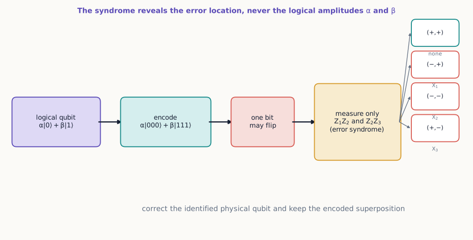
Figure 4:The repetition code stores logical information nonlocally. Two joint parity checks distinguish the four error locations but take the same values on both terms of the encoded superposition, so they reveal no information about or .
Concept check 12.4
In Example 12.3, a measured syndrome is . Which physical qubit has a bit flip, and has this measurement revealed anything about or ?
Answer
Qubit 2. The table shows occurs only for the row. The amplitudes are not revealed: the same syndrome occurs for the term and the term of the corrupted codeword, so the measurement distinguishes only which error occurred, not the encoded superposition.
Fault tolerance is the architecture that prevents imperfect correction operations from spreading errors uncontrollably. A scalable device needs error rates, connectivity, control, decoding, and overhead that together support logical operations—not merely a large physical qubit count.
Concept check 12.5
Is a larger number of physical qubits alone evidence of a more capable quantum computer?
Answer
No. Fidelity, connectivity, coherence, leakage, control speed, measurement, error correction, and algorithmic overhead all affect useful logical capability.
12.6 Quantum computation
A quantum algorithm uses interference so that amplitudes of unwanted answers cancel while amplitudes of useful outcomes reinforce. Superposition alone does not provide all answers to a problem: a final measurement returns one classical record, and the circuit must arrange that useful records have high probability.
Entangling gates plus arbitrary one-qubit rotations form a universal control set. Computational advantage is problem-dependent. Known examples exploit structure in integer factoring, quantum simulation, and some search or linear-algebra tasks; they do not imply a speedup for every computation.
When assessing an algorithmic claim, ask:
What input is loaded, and at what cost?
Which operations are assumed available?
How do time, qubit count, precision, and error-correction overhead scale?
What classical baseline is used?
What measurement produces the promised answer?
Example 12.4: Deutsch’s algorithm
Let be constant () or balanced (), with access to only through the oracle . Classically, deciding which case holds requires evaluating at both inputs. One query suffices quantum mechanically.
Prepare and apply :
Because the second qubit is , applying to one term reproduces the same two-term state up to an overall sign:
This is phase kickback: the oracle leaves the target qubit unchanged and writes into a sign attached to instead of into the target qubit’s state. Applying it to both terms gives
If is constant, the first factor in equation (13) is , an overall phase times ; a final on the first qubit returns with certainty. If is balanced, the first factor is , an overall phase times ; the final returns with certainty. Measuring the first qubit therefore reveals whether is constant or balanced—a single global property—after exactly one query to , even though neither nor separately becomes known. That one measured bit is direct evidence distinguishing the two hypotheses, not merely a result consistent with both. Nothing here followed one branch more than the other with higher probability; the two branches instead interfered constructively for one final measurement outcome and destructively for the other, exactly the mechanism named at the start of this section.
Figure 5:Build this circuit on two wires: Hadamard both qubits, insert an oracle, then Hadamard the first qubit again before measuring it. All four possible oracles are built from gates already in the palette—identity or on the target qubit for a constant , and CNOT (with an extra for the other balanced case) for a balanced . Confirm the first qubit always reads 0 for the constant oracles and 1 for the balanced ones.
Interactive simulation: Qubit Sketch
Concept check 12.6
After running Deutsch’s algorithm in Example 12.4 and measuring the first qubit, do we know the value of ?
Answer
No. Only the global constant-or-balanced property is determined. The individual values and remain unknown from that one run—the algorithm answers a question about the function as a whole, not about any particular input.
12.7 Clocks, resonance, and sensing
The Ramsey sequence of Chapter 4 compares a controlled oscillator with a quantum transition frequency. Feedback steers the oscillator toward the center of the fringe, forming the basis of atomic clocks.
Magnetic resonance uses precession and pulses to infer magnetic fields and local environments. In nuclear magnetic resonance and magnetic-resonance imaging, spatially varying fields connect resonance frequency and phase to position. The measurable signal is an ensemble response, but its building blocks are the rotations, phases, and projections developed for one spin.
A two-state sensor accumulates phase
A final analyzer converts into a probability. Sensitivity improves with phase-accumulation time until decoherence reduces contrast. Pulse sequences can reject slowly varying unwanted fields or select a narrow frequency band.
Example 12.5: projection noise
If a binary readout has probability , independent trials estimate it with standard deviation
Near the steepest point of an interference fringe, probability uncertainty becomes phase uncertainty. Repeating four times as many independent trials improves this standard quantum scaling by a factor of two. Entangled sensor states can alter the scaling under ideal conditions, but state preparation, loss, and decoherence determine whether the advantage survives.
12.8 Quantum simulation
Quantum systems are often difficult to simulate classically because the state space dimension grows exponentially with subsystem count. A controllable quantum device can encode another Hamiltonian and measure its dynamics.
Two broad strategies are:
digital simulation, which decomposes evolution into gates; and
analog simulation, which engineers a physical Hamiltonian with the same relevant structure as the target.
Validation remains essential. Conservation laws, small instances accessible to classical calculation, symmetry checks, and measurements in multiple bases help distinguish target physics from control error.
12.9 Reading claims with the textbook’s framework
Every quantum technology can be analyzed with four questions:
Preparation: Which density operator is actually produced?
Transformation: Which Hamiltonian, channel, or gate acts, and for how long?
Measurement: Which observable or generalized detector record is read?
Evidence: Which statistics distinguish the quantum model from noise or a classical alternative?
Terms such as superposition, entanglement, and quantum advantage name specific mathematical and experimental resources. They should lead to testable probability distributions, not serve as substitutes for a mechanism.
Summary
Qubits are physical two-state systems controlled with unitary gates and projective measurements.
Linearity forbids universal cloning of an unknown state.
Entanglement plus classical communication enables teleportation and dense coding without faster-than-light signaling.
Decoherence arises when uncontrolled correlations hide phase information from a subsystem.
Error correction protects logical amplitudes by measuring error syndromes that reveal which error occurred without collapsing the encoded state.
Phase kickback lets an oracle mark a global property of a function in the phase of a query register, letting interference answer a global question with fewer queries than any classical algorithm, as in Deutsch’s algorithm.
Computation, sensing, clocks, resonance, and simulation all use controlled preparation, phase evolution, interference, and readout.
Exercises
Find the action of , , and on each computational basis state and on .
Show that CNOT applied to does not produce two copies unless the first state is a computational-basis state.
Derive the teleportation identity by expanding both sides in the computational basis.
Make a table of the four Bell-measurement outcomes and the receiver’s correcting gate.
Work through superdense coding for all four two-bit messages.
Trace out the environment in the decoherence model and show that the off-diagonal terms are multiplied by .
Show how a single bit flip affects each codeword of the three-qubit repetition code and propose parity checks that locate it.
Explain why measuring every physical qubit directly would destroy the logical superposition even though syndrome measurements need not.
For , find and identify its steepest operating points.
A sensor has contrast , so . Explain how and affect small-field sensitivity.
Compare the resources consumed by teleportation, superdense coding, and direct qubit transmission.
Choose one quantum-technology claim and analyze it using the four questions in Section 12.9.
Suppose a unitary satisfies the cloning hypothesis for two states with . Show that equation (4) requires , and state which assumption fails.
Redo Example 12.1 for the Bell-measurement outcome instead of : find qubit 3’s state before correction and the operator order that recovers exactly.
For and , find the number of gates, run back to back, after which the coherence factor first falls below 0.5.
Verify directly, as in Example 12.3, that an error gives the syndrome .
A phase-flip error acts on . Show that both stabilizers and still return +1, and explain what this implies about the limits of the bit-flip code stated in the text.
Work through the phase-kickback calculation of Example 12.4 explicitly for the balanced assignment , tracking the overall phase, and confirm that the first qubit is still measured to be 1.
Suppose the target qubit in Deutsch’s algorithm were prepared in instead of , so no state is created. Show that then leaves the target entangled with the first qubit’s basis states, and explain why the final measurement on the first qubit no longer reliably distinguishes constant from balanced .
The Deutsch–Jozsa algorithm generalizes Example 12.4 to , promised to be constant or balanced, distinguished with one query using query qubits and the same target-qubit trick. Explain qualitatively, without a full derivation, why the phase-kickback mechanism still applies with query qubits and why a classical deterministic algorithm can require up to queries in the worst case.
Using the orthonormality of the Bell basis and of , verify that the four terms on the right of equation (5) are mutually orthonormal, and explain why this is required for the identity to represent a valid change of basis.
A vendor claims a -physical-qubit device demonstrates “exponential quantum advantage” on an optimization problem. Apply the four questions of Section 12.9 to list the specific information needed before evaluating the claim.
Using the per-gate coherence factor from Example 12.2, estimate how many gates a device could run before losing half its coherence, and compare this with the -gate estimate already given in the text.
Explain, using the vocabulary introduced across Sections 12.3–12.5 (preparation, transformation, measurement, evidence), what distinguishes a genuine demonstration of quantum error correction from one that merely shows a syndrome-measurement circuit runs without crashing.