Approximation methods
Learning objectives
After this chapter, you should be able to:
calculate first- and second-order stationary perturbation corrections;
handle a perturbation inside a degenerate subspace;
apply the variational principle to estimate a ground-state energy;
identify the semiclassical regime and use WKB connection ideas;
calculate first-order transition amplitudes from a time-dependent perturbation; and
judge an approximation using dimensionless parameters and limiting cases.
10.1 Why approximations are part of the theory
Exactly solvable Hamiltonians are rare. Real atoms interact with fields and other particles; real wells are not perfectly square; and most coupled differential equations do not have closed-form solutions. Approximation methods are controlled ways to retain the most important physics.
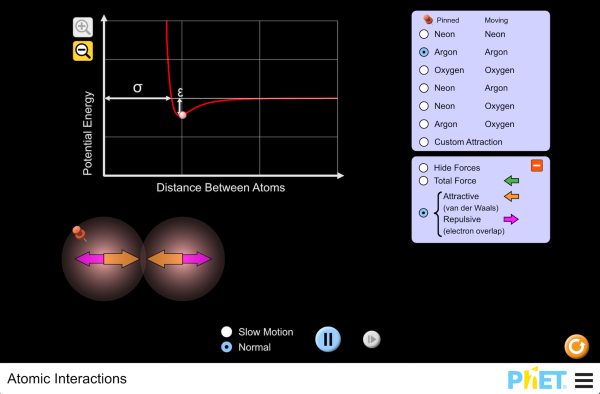
Figure 1:The interaction between two real atoms is not a square well or a harmonic oscillator; it is closer to the Lennard-Jones potential this simulation plots. Adjust the atom types and separation and watch the force and potential energy curves change shape—exactly the kind of realistic potential the methods below are built to handle without an exact solution.
Interactive simulation: Atomic Interactions
Before calculating, identify a dimensionless small or large parameter. An answer labeled “first order” is useful only when omitted terms are expected to be smaller. After calculating, check normalization, units, symmetry, and the limit in which the perturbation disappears.
This chapter develops five complementary tools. Stationary perturbation theory (Sections 10.2–10.3) corrects the energies and states of a Hamiltonian that is close to one already solved. The variational principle (Section 10.4) needs no such reference Hamiltonian at all, only a plausible guess for the shape of a ground state. WKB (Section 10.5) exploits a different smallness—a slowly varying potential rather than a weak one—and applies even when no nearby solvable problem exists. Time-dependent perturbation theory (Section 10.6) answers a different question altogether: not “what is the corrected energy” but “what is the probability of a transition.” Section 10.7 collects these into a single decision procedure. None of the five methods is a substitute for solving the Schrödinger equation exactly; each is a controlled bookkeeping scheme for what happens when an exact solution is out of reach.
10.2 Nondegenerate stationary perturbation theory
Let
where is solved and tracks order. Expand
and similarly for the ket. Matching powers of gives
and
The first energy correction is the perturbing potential averaged in the unperturbed state. State mixing is large when a coupling matrix element is large or an energy denominator is small.
Example 10.1: a two-level perturbation
Take
The diagonal matrix elements of vanish, so both first-order energy shifts vanish. For the upper level,
while . Expanding the exact eigenvalues confirms these results. Comparison with an exact answer is an excellent way to understand an approximation’s domain.
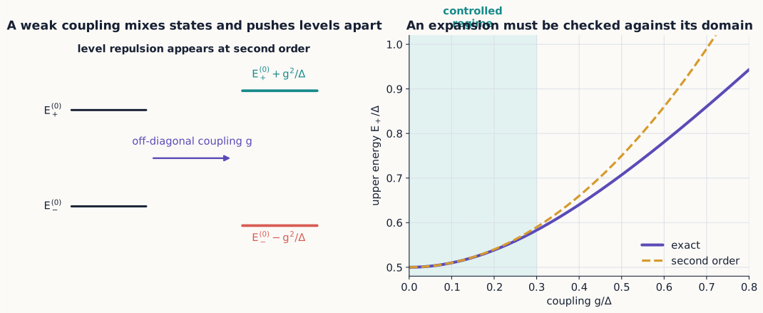
Figure 2:Off-diagonal coupling produces level repulsion even when the first-order diagonal shifts vanish. The truncated series follows the exact answer only while the coupling remains small relative to the unperturbed gap.
Selection rules save work
If symmetry forces , that state does not appear in the corresponding sum. For example, an odd perturbation has zero diagonal matrix element in a parity eigenstate, so its first-order energy shift vanishes. A zero correction often expresses symmetry, not absence of a physical effect at every order.
Concept check 10.1
Can a first-order correction vanish while the exact energy still changes?
Answer
Yes. Symmetry may make the diagonal matrix element zero while second- and higher-order corrections remain.
Example 10.2: an anharmonic correction that grows with the state
Take the harmonic oscillator of Chapter 7, , perturbed by a quartic term with strength , so . When we write and expand , only terms that return to survive the diagonal matrix element, and their combinatorics give
Two features are worth pausing on. First, unlike Example 10.1, no diagonal matrix element vanishes here—the quartic term is even, like the unperturbed potential, so nothing forbids a first-order shift. Second, and more important, the correction is not a fixed small number: it grows quadratically with . A denominator or matrix element being “small” is a statement about one particular calculation, not a permanent property of .
Concept check 10.2
For the quartic oscillator of Example 10.2, does making smaller guarantee that first-order perturbation theory is accurate for every level ?
Answer
No. Equation (8) grows like for fixed , so for any nonzero there is always some large enough at which the correction rivals the level spacing . Making smaller only pushes that breakdown to higher ; it does not remove it.
10.3 Degenerate perturbation theory
Equation (4) fails when a denominator vanishes: dividing by is not a small correction but a breakdown of the expansion. Whenever two or more unperturbed states share an energy, the zeroth-order states are not yet uniquely determined—any combination within the degenerate subspace is equally an eigenstate of —and the perturbation itself must be used to select the right combination before a first-order energy shift means anything. Within a degenerate subspace, first diagonalize the matrix
Its eigenvectors are the correct zeroth-order combinations, and its eigenvalues are their first-order energy shifts.
Example 10.3: splitting a degenerate pair
Suppose and both have energy , and within their subspace
The shifts are . If , corresponding normalized states can be chosen as
The perturbation both selects a preferred basis and lifts the degeneracy.
10.4 The variational principle
Sections 10.2 and 10.3 both correct a Hamiltonian that is already close to a solved one. The variational principle needs no such reference Hamiltonian: it converts a guess about the general shape of a ground state directly into a number, at the price of no longer knowing how close that number is to the truth without further work.
For a Hamiltonian bounded below, any normalized trial state obeys
Expanding the trial state in exact energy eigenstates proves the result: . Varying parameters in a sensible trial family gives the best upper bound available within that family.
Example 10.4: estimate a confined ground state
For a one-dimensional Hamiltonian
choose the normalized Gaussian
Its energy is
Minimizing balances localization kinetic energy against potential energy and determines both an energy upper bound and an approximate spatial scale. Dimensional analysis already predicts .
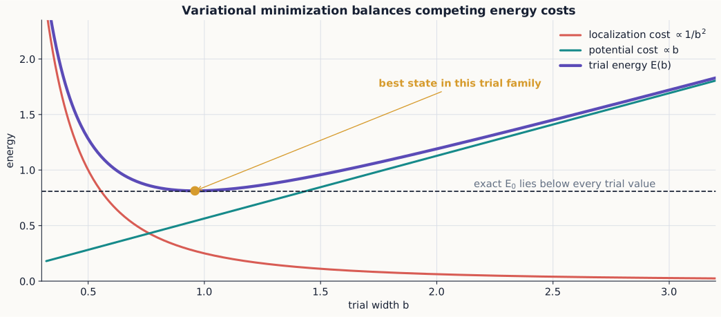
Figure 3:Variational optimization balances competing costs: a narrow state pays high kinetic energy, while a broad state samples more potential energy. The minimum is the best upper bound supplied by the chosen family, not necessarily the exact ground energy.
The variational method is safest for the ground state. The reason is worth making explicit rather than taking on faith. Expanding any normalized trial state in the exact eigenbasis, , gives , a weighted average of all the exact energies with nonnegative weights summing to one. Such an average can never fall below the smallest term , which is exactly equation (12). There is no equally automatic bound relative to the first excited energy : nothing stops a trial state from having some overlap with the true ground state, which pulls below without violating anything. Excited-state estimates therefore require trial functions built to be exactly orthogonal to the true ground state—typically enforced by symmetry, such as parity or a node structure, rather than by numerically minimizing overlap. If the exact ground state is not fully known, an excited-state trial function orthogonal only to an approximate ground state offers no guaranteed bound at all.
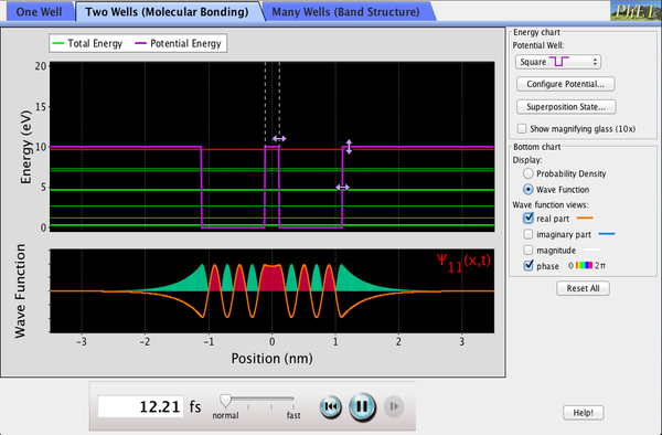
Figure 4:Build a well and read off its ground-state energy directly, then compare that exact number against the trial-Gaussian estimate from equation (12)—the same simulation introduced for the finite well in Chapter 7, now used to check a variational guess rather than to explore an exactly solvable potential.
Interactive simulation: Bound States
Concept check 10.3
Why is a variational energy below a known exact ground energy a warning?
Answer
For a normalized trial state and the correct Hamiltonian it is impossible. Such a result signals an algebra, normalization, boundary-condition, or numerical error.
10.5 The WKB approximation
The variational principle traded a small parameter for a guessed function shape. WKB reintroduces a small parameter, but a geometric one: not a weak coupling, but a potential that varies slowly compared with the local de Broglie wavelength. Write a stationary wavefunction locally as
When the potential varies slowly over a local wavelength, the leading semiclassical solution in an allowed region is
where . In a forbidden region, set to obtain growing and decaying exponentials.
Across a broad forbidden region , the leading tunneling factor is
For bound motion between two smooth turning points, connection formulas give
WKB fails near a turning point if used without connection formulas and fails when the potential changes substantially within one wavelength.
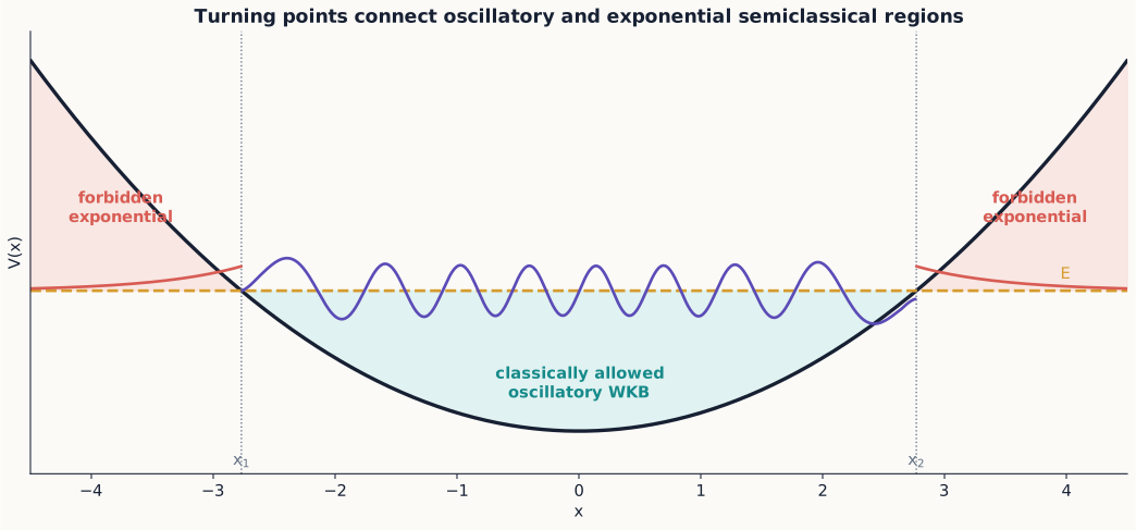
Figure 5:Turning points divide oscillatory, classically allowed motion from exponential, forbidden behavior. Connection formulas—not the separate local expressions—are what carry one approximation smoothly into the other.
Concept check 10.4
Does WKB require high total energy in every problem?
Answer
No. It requires the wavelength to vary slowly on the wavelength scale. High energy often helps, but slowly varying potentials can also create a valid semiclassical regime.
Example 10.5: the quantum bouncer
A particle of mass rests above an impenetrable floor under a uniform downward force : for and for . This potential has only one smooth classical turning point, at ; the other boundary is not a turning point at all but a hard wall, where the exact wavefunction must vanish outright rather than decay smoothly.
Equation (19) was derived for two smooth turning points, each contributing a connection-formula phase of . Standard connection-formula analysis shows that a hard wall contributes instead, since the wave is forced to a node exactly at the wall rather than merely turning around over an extended region. Replacing one by changes the quantization condition to
With , substituting gives
Solving equation (20) for gives
so for large . Two features distinguish this spectrum from the harmonic oscillator of Chapter 7: the energies grow as rather than linearly, so the fractional level spacing shrinks as grows instead of staying fixed. WKB reaches this result without ever constructing the bouncer’s exact Airy-function wavefunction—a genuine payoff of the method beyond the textbook-symmetric wells where an exact solution is available for comparison.
Concept check 10.5
Why isn’t the quantum bouncer’s quantization condition the same rule used for the harmonic oscillator?
Answer
The oscillator has two smooth classical turning points, each contributing a connection-formula phase of , for a total of . The bouncer has one smooth turning point and one hard wall; the wall enforces an exact node and contributes by itself, for the same total phase but a different split, giving the condition of equation (20).
10.6 Time-dependent perturbations
Stationary perturbation theory and the variational method both estimate properties of energy eigenstates. Time-dependent perturbation theory asks a different kind of question: given a system prepared in one eigenstate of , with what probability does a time-dependent coupling later find it in another? Let
Starting in , the first-order amplitude to find is
Example 10.6: a coupling switched on and held constant
The simplest case is a time-independent matrix element switched on suddenly at and left constant afterward. Equation (24) then integrates directly:
Taking and using gives
At exact resonance, , this reduces to : the probability grows without bound as , a reminder that first-order perturbation theory is itself only a short-time approximation and must break down—by unitarity, cannot exceed one—before grows too large. Away from resonance, equation (26) oscillates in without growing, confined between 0 and .
Viewed as a function of at fixed , equation (26) is a single central peak of height and width (first zero) at , surrounded by decaying side lobes—the same line shape that appears in single-slit diffraction. The peak narrows as while its height grows as ; a longer observation window makes the transition simultaneously more probable at exact resonance and more sharply selective in energy. This time–frequency trade-off is what allows the discrete result of this example to reproduce the smooth, irreversible-looking rate of equation (27) once many closely spaced final states are summed over.
Concept check 10.6
Does making the interaction time longer in Example 10.6 make a transition more or less selective in energy?
Answer
An oscillating perturbation contains phases . The integral grows most strongly when the driving frequency is near : resonance is constructive accumulation of transition amplitude over time.
For a long interaction and a dense set of final states, the transition rate often takes the form
known as Fermi’s golden rule. The density of available final states matters alongside the coupling strength.
10.7 Choosing and checking a method
Use stationary perturbation theory for weak changes to known discrete eigenstates, degenerate perturbation theory when small denominators signal a degenerate subspace, the variational method for ground-state bounds, WKB for slowly varying potentials or semiclassical tunneling, and time-dependent perturbation theory for weakly driven transitions.
An approximation should report:
the parameter assumed small or large;
the order retained;
the symmetry restrictions used;
the range where the expression is expected to work; and
at least one independent check.
Summary
Perturbation theory organizes corrections in powers of a small coupling, but “small” must be checked state by state: a fixed coupling can produce an arbitrarily large correction at a high enough quantum number.
Degenerate spaces must be diagonalized before nondegenerate formulas apply.
The variational principle gives an upper bound to the ground energy for any normalized trial state; the same guarantee does not extend to excited states without enforced orthogonality to the true ground state.
WKB describes slowly varying waves, semiclassical quantization, and exponential tunneling; a hard wall and a smooth turning point contribute different phases to the same connection formula.
Time-dependent perturbations create transitions by coherent amplitude accumulation, especially near resonance, and a longer interaction time trades a broader, weaker response for a narrower, more resonance-selective one.
Every approximation needs an explicit control parameter and validity check.
Exercises
Expand the exact eigenvalues in Example 10.1 through fourth order in .
For an infinite well perturbed by , calculate the first-order energy shift.
Use parity to decide which matrix elements connect even and odd states for even and odd perturbations.
Diagonalize the matrix in Example 10.3 and verify its phase-dependent eigenvectors.
Minimize the trial energy in Example 10.4 and give the numerical coefficient multiplying its natural energy scale.
Prove the variational bound by expanding a normalized trial state in exact eigenstates.
Apply equation (19) to the harmonic oscillator and recover its exact energies.
Show that equation (18) reduces to the exponential part of the rectangular-barrier result.
Redo the calculation of Example 10.6 for a matrix element that is switched on at and switched off again at , remaining zero afterward. Find for and compare with equation (26) evaluated at the same total “on” time.
State which approximation method is best suited to four scenarios: a weak Stark shift, a ground energy of an anharmonic well, alpha decay, and weak resonant light absorption.
Identify a dimensionless validity parameter for each method used in this chapter.
Verify equation (8) for and directly, by expanding in normal-ordered form and evaluating each surviving term between and .
For fixed small in Example 10.2, find the quantum number at which first becomes comparable to the unperturbed spacing . Explain why depends on even though is “small” by assumption.
A perturbation (linear, not quadratic) is added to the harmonic oscillator. Show that first-order perturbation theory predicts a zero energy shift at every level, then find the exact shifted spectrum by completing the square in the full Hamiltonian, and explain why the “vanishing” first-order result is not a contradiction.
Using the eigenstate-expansion argument of Section 10.4, explain why no two normalized trial states can both give an expectation value strictly below the true ground energy of the same Hamiltonian.
Give a concrete example of a trial state that is exactly orthogonal to an approximate (numerically obtained, not exact) ground state, and explain why minimizing its energy need not bound the true first excited energy from above.
Derive the classical turning point and the WKB integral for the quantum bouncer of Example 10.5, and confirm both the quantization condition (20) and the resulting scaling .
Compare the quantum-bouncer energies at and using equation (22): by what factor does the energy increase? Does the fractional spacing grow or shrink with ?
Explain, in terms of the boundary condition on the wavefunction, why a hard wall and a smooth classical turning point contribute different phases to a WKB connection formula.
Starting from equation (24), rederive equation (26), and show that it reduces to in the limit .
Show that the peak value of equation (26) grows as while its width in shrinks as , so that the area under the peak approaches a constant. Explain in one sentence how this supports treating the transition rate as time-independent once many closely spaced final states are summed, as in equation (27).
A perturbation is switched on with a smooth ramp instead of the abrupt step used in Example 10.6. Without repeating the full integral, explain qualitatively how a smoother switch-on changes the side lobes of the line shape far from resonance.
For each of the five methods developed in this chapter, write one sentence describing the physical situation where it is the natural first method to try, and a second sentence describing a warning sign—in the setup or in the answer—that the method has been pushed past its domain of validity.