Operators and measurement
Learning objectives
After this chapter, you should be able to:
represent observables by Hermitian operators;
calculate eigenvalues, eigenvectors, and spectral decompositions;
apply the Born rule and the projection postulate;
compute expectation values and uncertainties;
use commutators to diagnose incompatible observables;
reconstruct a spin state from component-measurement statistics;
use Pauli-matrix identities to simplify spin calculations; and
represent pure states, mixtures, and unread measurements with density operators.
Sections 3.8 and 3.9 are optional mathematical extensions. They prove the spectral structure used earlier and collect compact Pauli identities, but the measurement and density-operator sections do not depend on completing every derivation there.
3.1 Observables as operators
Chapter 2 treated , , and every other spin component separately, building a fresh pair of basis kets each time we wanted to ask a new question. That approach works, but it is repetitive: the same idea—“measure spin along some axis”—kept reappearing with different labels attached. It is both more efficient and more revealing to package that whole idea into a single mathematical object, called an operator. Its eigenvalues list the possible outcomes, and its eigenspaces identify the states that make those outcomes certain. Applying the operator to an arbitrary ket is an algebraic operation, not a literal simulation of one laboratory measurement.
A physical observable is represented by a Hermitian linear operator: one equal to its own conjugate transpose. Section 3.8 will show exactly why this property is what guarantees real, physically sensible measurement outcomes; for now, treat it as the defining requirement an operator must satisfy to represent something measurable. For spin , it is convenient to introduce the Pauli matrices
The spin operators are built directly from them:
Hermiticity, written , guarantees two things at once: real eigenvalues, and an orthonormal eigenbasis. These are exactly the two properties we need from an ideal measurement: real numbers on a meter, and a definite state associated with each possible reading.
For example, applying to the two basis kets just returns them, scaled by the corresponding measured value:
It is worth stressing what the possible measured values actually are: they are the eigenvalues of the operator, not just any numbers that happen to appear when we write out its matrix in some basis.
One apparatus, three mathematical objects
For an ideal measurement, it helps to keep three related objects distinct, since students often blur them together at first:
| Laboratory meaning | Mathematical object | For |
|---|---|---|
| A possible detector reading | eigenvalue | or |
| A state that makes that reading certain | eigenket | $ |
| The test for membership in that outcome state | projector | $ |
The observable operator packages all three pieces of information into one object. Solving its eigenvalue equation
extracts the possible readings and the corresponding definite-outcome states in one stroke. The prepared state need not itself be one of those eigenkets; in general, it will not be. Instead, its projections onto them are what determine the outcome probabilities, as the next section makes precise.
3.2 Constructing an operator from its measurement states
We can build an operator representing a measurement directly out of its outcome states, using a tool already implicit in Chapter 2’s basis expansions: the projector. A projector is an operator that takes an arbitrary state, extracts its component along one particular direction in state space, and discards the rest. Define the projectors
Direct from the definition, they satisfy three properties: (projecting twice does nothing new), (each is Hermitian), and (the two outcomes are mutually exclusive). Because the two basis states span the space, . This is the operator form of the basis expansion used in Chapter 2.
Combining the eigenvalues with their projectors reconstructs the full operator. The spectral decomposition of is
More generally, if a Hermitian observable has nondegenerate eigenstates and eigenvalues , the same pattern holds for any number of outcomes:
This expression cleanly separates two pieces of information that are easy to conflate: the possible values , and the state projectors associated with those values.
Example 3.1: construct 
Using equation (20),
The last matrix is written in the basis. In the basis, the same operator is diagonal—a reminder that “the matrix of an operator” always means the matrix in a particular basis, never an absolute property of the operator alone.
This construction also runs in reverse: if the matrix of an observable is already known, its eigenvectors identify the corresponding analyzer states. This two-way connection deserves practice in both directions:
Keep in mind what the operator is not. It is not an additional physical substance carried around by the atom. It is simply the linear map that encodes one particular experimental question—nothing more, and nothing less.
Concept check: reading a spectral decomposition
In , which symbols denote detector readings, definite-outcome states, and tests for the two outcomes?
Answer
The numbers are detector readings; the kets are definite-outcome states; and the projectors test for those outcomes.
3.3 Measurement probabilities and state update
For a system prepared in , the probability of obtaining result follows directly from the Born rule of Chapter 2, now written using the projector language just introduced:
If is obtained in an ideal nondegenerate measurement, the state immediately after the measurement is , up to an overall phase. This is the projection postulate: before the result is known, the theory supplies a probability distribution over outcomes; the instant a result is selected, that same theory supplies a new preparation to use going forward.
A reusable measurement workflow
Given a prepared state and an observable, the same five steps apply every time:
Diagonalize the observable if its eigenvalues and normalized eigenkets are not already known.
Build the projector for each distinct outcome.
Compute and check that the probabilities sum to one.
If an outcome is selected, apply its projector and normalize the result.
Use the resulting state—not the original state—for any later measurement.
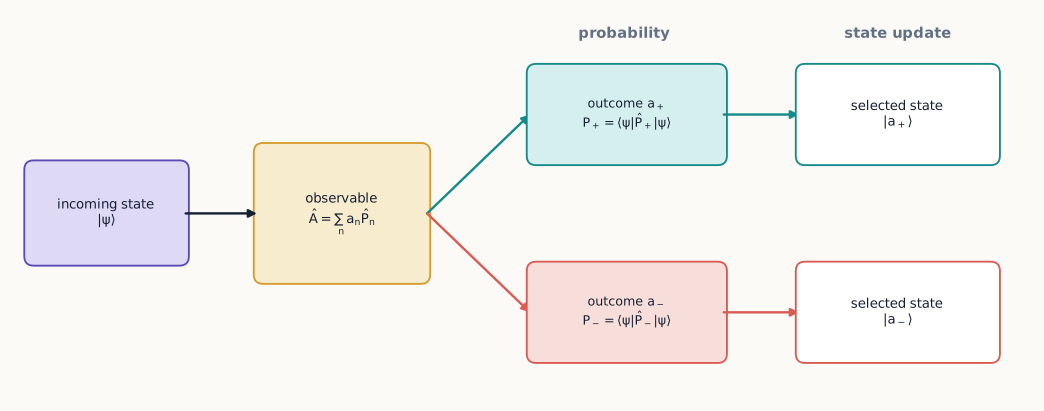
Figure 1:A projective measurement does two jobs. Its spectral projectors determine the probabilities of the possible records, and a selected record supplies the state used in every later step.
This workflow is nothing more than the operator version of tracing a route through sequential Stern–Gerlach analyzers, which Chapter 1 did by hand and Chapter 2 did with explicit amplitudes.
Example 3.2: measure along a tilted axis
Let lie in the plane. In the basis,
Its normalized eigenket can be chosen as
For a input,
The operator method has recovered the same half-angle rule found empirically in Chapter 1, while also identifying the exact state prepared once the result is selected, something the earlier probability-tree approach could not supply on its own.
This projector construction also makes repeatability, Chapter 1’s first empirical rule, mathematically transparent. For a one-dimensional outcome space,
because . Reading this equation in words: applying the same projector a second time changes nothing. A second immediate measurement therefore finds the same outcome with certainty. This is an important consistency check on the projection postulate: once ideal measurement has been modeled by a projector update, repeatability follows from idempotence. The algebra does not derive the update rule from the Born rule; the update itself remains part of the ideal-measurement postulate motivated by the experiments of Chapter 1.
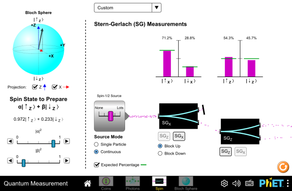
Figure 2:Prepare a spin- state, choose an analyzer orientation , and watch the projection postulate act: a Bloch-sphere readout shows the prepared state collapse to the instant a result is recorded. Reproduce Example 3.2 by tilting the analyzer to angle from a preparation and comparing the displayed probability with .
Interactive simulation: Quantum Measurement: Spin
3.4 Expectation values
A single measurement returns one eigenvalue, chosen randomly according to the Born-rule probabilities. It is also useful to ask a different question: what would the average reading be, over many repetitions of the same preparation and measurement? This is a number a laboratory can compare directly to a meter that reports a running mean, rather than a single random outcome. We call it the expectation value, and it is the ensemble average predicted for many identically prepared systems:
An important subtlety: the expectation value need not itself be a possible result of any single measurement. For spin , is a perfectly good ensemble average even though no individual measurement can ever return zero: every single measurement returns or .
Example 3.3: mean spin
Let . Then
For the Bloch-sphere state of equation (45), this becomes
Repeating the same calculation for and gives the complete result
So the Bloch vector points along the expectation value of spin. Be careful not to overread this: it does not mean every component simultaneously has that value in any single measurement, only that this is the value each component averages to.
Expectation values as state tomography
For a spin- pure state, the three mean Pauli components together determine the Bloch vector completely:
Each component is measured experimentally from counts, not read off directly. If and are the numbers measured on identically prepared members of an ensemble, then
with analogous expressions for and . Three separate subensembles are required, one per axis, because the three spin components cannot all be measured sharply on the same atom: measuring one disturbs what can be known about the others. The general process of reconstructing a state from a collection of measurement statistics like this is called quantum-state tomography.
For a pure state, exactly. Values with describe mixed states, which Section 3.10 introduces properly; the completely unpolarized mixture sits at . So “zero mean spin” does not, by itself, mean that every measurement returns zero—indeed, zero is not even an allowed result for a single spin- component measurement.
3.5 Variance and uncertainty
Just as the expectation value captures the center of a distribution of outcomes, we also want a number that captures its spread. The variance of is defined, as in ordinary statistics, by
For every spin component, , a fact that follows directly from . Applying this to a state gives
Zero uncertainty means exactly one thing: the state is an eigenstate of the observable in question. It does not mean that all observables are simultaneously sharp: here is perfectly definite while and are maximally spread.
Concept check 3.1
If , must the state have a definite value of ?
Answer
No. Every equatorial Bloch-sphere state has , but only two of them, and , have definite .
Concept check 3.2
Can an expectation value lie outside the range of an observable’s eigenvalues?
Answer
No. It is a probability-weighted average of the eigenvalues. It can lie between them, even when that intermediate value cannot occur in one measurement.
For an arbitrary component in a pure state with Bloch vector , the two possible outcomes immediately give both the mean and the spread in closed form:
The uncertainty vanishes precisely when the analyzer points along or opposite the Bloch vector, and it is maximal for every direction perpendicular to it. This is the cleanest way to see that uncertainty is a property of a state relative to a specified measurement—not some intrinsic fuzziness of the state considered alone.
Concept check 3.3
A student calculates in a state . What can be concluded about ?
Answer
It must be an eigenstate of , so it is or up to an overall phase. The calculation does not imply zero uncertainty for or ; each of those uncertainties is .
3.6 Commutators and incompatibility
Chapter 1 showed experimentally that measuring then gives a different final distribution than measuring then : order matters for incompatible observables. We now want a single algebraic object that captures this order-dependence directly, without having to redo the Stern–Gerlach bookkeeping every time. The commutator of two operators is
If and commute, the order in which we apply them makes no difference; if the commutator is nonzero, order matters. It is worth multiplying the Pauli matrices out by hand once, so that the result is not taken purely on faith. Using equation (2),
while multiplying in the opposite order gives
The two products are not equal—already a direct demonstration that matrix multiplication need not commute—and their difference is . Inserting from equation (3) then gives
with cyclic permutations for the other pairs, obtained by the same steps with relabeled throughout. This nonzero commutator is the precise algebraic counterpart of the sequential-analyzer behavior observed in Chapter 1.
The commutator also controls how sharply two observables can be simultaneously known. For any state,
In a state, equation (30) gives ; both uncertainties equal , so the bound is saturated exactly—there is no slack left.
The right-hand side is state dependent. A nonzero commutator operator does not guarantee a positive numerical lower bound in every state. For example, in ,
so Robertson gives only . The observables are still incompatible; this particular bound is merely uninformative for this state. Indeed and . Noncommutation is an operator statement, whereas the numerical lower bound also depends on the preparation.
Noncommutation is closely related to analyzer order, but be careful not to equate an operator product directly with “perform one projective measurement and then the other.” A selected sequence also includes a state update in between, which the bare commutator does not track by itself. For example, the route probability for is
Reversing the two projectors changes the physical route being described: it answers a different experimental question, not just a reordered version of the same one. The projector product keeps both the ordering and the conditional selection explicit, which the commutator alone does not.
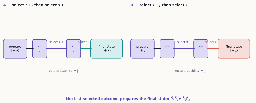
Figure 3:Reversing two selected measurements reverses which eigenstate is prepared last. Even when the displayed routes happen to have equal probabilities, their final states differ: and are not the same operation.
3.7 Operators along an arbitrary direction
For a unit vector , define the spin component along that direction as
Its eigenvalues are , for any choice of , a fact consistent with Chapter 1’s observation that every analyzer, no matter how it is oriented, gives exactly two outcomes. Its eigenstate is the Bloch-sphere state in equation (45), up to an overall phase. The compact identity
makes the eigenvalues immediate, without any further diagonalization.
The associated outcome projectors can be written down directly, without first solving for the eigenvectors at all:
They sum to the identity, as any pair of complementary projectors must, and satisfy . For a state with Bloch vector , equation (35) yields a compact probability rule that is often faster to use than working with explicit eigenkets:
This is the operator version of equation (49), and it remains useful even for mixed states, whose Bloch vectors lie strictly inside the sphere rather than on its surface.
3.8 Optional extension: why Hermitian operators have the needed structure
Section 3.1 asserted that Hermiticity guarantees real eigenvalues and orthogonal eigenstates. It is worth proving both claims directly because they explain why Hermitian operators fit ideal observables in finite-dimensional quantum mechanics.
Suppose
for a normalized eigenket. Taking the inner product with gives
For a Hermitian operator, complex-conjugating this expression and using gives
so , meaning the eigenvalue is real. This is precisely what we need: detector readings can be real numbers with physical units, not complex quantities with no direct meter reading.
Now let and have distinct eigenvalues and . Hermiticity gives
but also, moving to act on the bra instead,
Subtracting these two expressions for the same quantity gives . If , the only way this can hold is : states belonging to distinct ideal outcomes are automatically orthogonal. In a degenerate eigenspace, where several states share one eigenvalue, orthonormal eigenvectors can still be chosen within that subspace, but the measurement outcome alone does not identify which particular vector within it was present.
Together these two facts give the finite-dimensional spectral theorem: every Hermitian operator has an orthonormal eigenbasis, and can be written
where projects onto the full eigenspace belonging to the distinct value . The nondegenerate formula already used in equation (8) is just the special case , where each eigenspace happens to be one-dimensional.
Example 3.4: diagonalize a two-state observable
Consider
The matrix is Hermitian because its off-diagonal entries are complex conjugates of each other. Its characteristic equation is
so the possible outcomes are the real values —real, exactly as Hermiticity guaranteed in advance.
A quick check catches most sign or arithmetic errors before going any further: the sum of the eigenvalues must equal the trace of , and their product must equal its determinant. Here , and , which indeed matches the determinant computed above, . Both checks pass, so it is safe to proceed.
To find the eigenvector for , write and use either row of : the two rows are not independent equations once is an exact root, so either one alone determines the ratio . The second row reads , so
Choosing gives a squared norm
so one normalized eigenket is
For , the second row instead gives when . Its squared norm is , so
Before trusting the result, check the inner product. The product of the two lower components before normalization is
which cancels the product of the upper components. Thus . We have now completed the full workflow: find the eigenvalues, solve for each component ratio, normalize, and check orthogonality. Hermiticity told us in advance that the roots would be real and that such an orthonormal eigenbasis must exist.
3.9 Optional extension: the Pauli algebra as a calculation tool
Many spin calculations become much shorter once a few Pauli-matrix identities are available, so they are collected here as tools rather than rederived from scratch each time. Direct multiplication of the matrices in equation (2) gives
Here is one when the indices agree and zero otherwise, while supplies the sign associated with a cyclic ordering of . Packaging all nine possible products into a single vector identity gives
Setting immediately recovers for a unit vector, without any further calculation. Subtracting the same formula with and exchanged—and using —gives the commutator for components along two arbitrary directions:
Parallel components commute, since their cross product vanishes; perpendicular components have the largest possible commutator magnitude. In this way, the vector geometry of analyzer directions is encoded directly in the operator algebra, rather than needing to be checked case by case.
Example 3.5: two projectors in succession
Using equation (35),
The imaginary cross-product term changes sign if the order is reversed, so the two operators are identical only for parallel or antiparallel axes; any other pair of directions gives an order-dependent result. Acting on and taking the squared norm yields , recovering the analyzer angle rule while also retaining the post-selected output state, something the bare probability number alone would not do.
3.10 Density operators and unread measurements
A ket describes a pure preparation: every atom in the ensemble was prepared exactly the same way. But real experiments sometimes involve a classical mixture of different preparations—an ensemble in which state occurs with classical probability . This is represented by the density operator
Recall that the trace of an operator is the sum of its diagonal entries in any orthonormal basis; the result does not depend on which basis is chosen. (This is the same fact used as a check in Example 3.4: the trace, computed from the diagonal entries, equals the sum of the eigenvalues, computed from an entirely different calculation.) A density operator is always Hermitian, has trace one, and has no negative eigenvalues. In this language, probabilities and expectation values take compact forms that work for pure states and mixtures alike:
For a pure state, and , so . A genuine mixture instead has . This purity test gives a single number that tells pure states and mixtures apart, and it does not depend on which basis we use to compute it.
Every spin- density operator, pure or mixed, can be written in Bloch-vector form:
Pure states lie exactly on the surface of the Bloch sphere, where ; mixed states lie strictly inside it. The completely unpolarized state sits at the very center, , and predicts equal probabilities for every possible analyzer orientation.
Example 3.6: tomography from three analyzer settings
Suppose three equal subensembles produce
Since for each axis,
Its length is exactly one, so this idealized data describes a pure equatorial state. A representative ket reproducing it is
In a real experiment, finite-sample noise means the reconstructed vector may come out slightly outside the unit sphere, with marginally greater than one. A statistically sound tomography method then finds the nearest physically allowed density operator, rather than trying to interpret as if it described a valid quantum state.
An outcome ignored is not a measurement undone
Here is a question that trips up many students on first encounter: if an ideal measurement occurs but nobody looks at the result, has anything changed? The answer is yes—and understanding why is one of the more important lessons in this chapter. If an ideal projective measurement occurs but its result is not retained, the post-measurement ensemble is
For an initial state followed by an unread measurement,
Notice what happened to the off-diagonal -basis terms: they have disappeared entirely. As a direct consequence, a later measurement is now 50–50, even though no observer ever actually used the intermediate result. Discarding a record after the fact is not the same as preventing that record from being created in the first place. It is the physical correlation that made the alternatives distinguishable—not anyone’s act of reading it—that destroyed the interference. This is exactly the distinction the quantum-coin-toss simulation of Chapter 2 makes tangible: a coin that has decohered into a fixed outcome behaves just like above, no matter whether that outcome has been read yet.
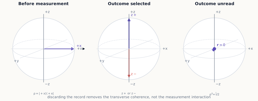
Figure 4:An measurement sends each member of the ensemble to a pole. Keeping the outcome selects one pole; pooling the outcomes leaves no net Bloch vector and removes the transverse coherence of the initial state.
Concept check 3.4
Can the same density operator arise from different preparation recipes?
Answer
Yes. For example, equal mixtures of and , of and , or of and all give . No measurement on the spin alone can distinguish preparation recipes that produce the same density operator.
Concept check 3.5
An unread measurement is made on a state. Does its density operator change?
Answer
No. Equation (60) returns and a zero contribution from the other projector. The state was already definite for the measured observable.
By contrast, if the result is retained, the conditional density operator is
Equations (60) and (62) distinguish two common laboratory instructions that are easy to conflate in words but behave quite differently: “measure and forget the result” versus “measure and select one result.”
Summary
Hermitian operators represent observables; their eigenvalues are possible outcomes and their eigenvectors are definite-outcome states.
Projectors give both outcome probabilities and post-measurement states.
An expectation value is an ensemble mean, not generally a single outcome.
Variance quantifies the spread of repeated measurements on identically prepared systems.
Noncommuting observables encode order dependence and uncertainty relations.
Projector products describe selected routes through sequential measurements.
The three mean Pauli components reconstruct a spin state’s Bloch vector.
Hermiticity guarantees real outcomes and orthogonal eigenspaces for distinct outcomes.
Density operators describe pure states and mixtures in one framework; unread measurements remove coherence in the measured basis.
Exercises
Exercises 1–7 build the essential operator, projector, and expectation-value skills. Exercises 8–14 consolidate sequential measurement and state reconstruction. Exercises 15–22 draw on the optional mathematical extensions or density-operator material. A first pass can therefore use 1–7, 10–12, 18, and 20–21 without treating the entire list as one assignment.
Find the eigenvalues and normalized eigenvectors of each Pauli matrix.
Verify the projector properties for and using explicit -basis matrices.
For , calculate , , and .
Calculate by direct matrix multiplication.
Show that for any unit vector .
Derive the projectors .
A state gives . Find and without first finding a ket.
Give an example showing that and can differ. Explain how the commutator measures the difference.
For , write the -basis matrix of and verify the proposed eigenvector in Example 3.2.
Starting with , calculate the state and probability associated with the selected route using a product of projectors.
An ensemble produces counts , , and on three equal subensembles. Estimate its Bloch vector and decide whether the data are approximately consistent with a pure state.
Derive equation (25) from the two outcome probabilities in equation (36).
Prove all three projector properties for equation (35): Hermiticity, idempotence, and orthogonality of the and projectors.
Compare the two route probabilities and . Explain why they answer different experimental questions even though they contain the same two projectors.
For Example 3.4, verify both eigenvalue equations with the normalized eigenkets given in the text, then reconstruct from its spectral decomposition.
Derive equation (51) by expanding both dot products and using equation (50).
Use equation (52) to calculate the commutator of components along and .
Find the density matrix and purity for a mixture containing with probability and with probability . Draw or describe its Bloch vector.
Show from equation (56) that .
Verify every line of the unread-measurement calculation for an initial state using explicit matrices.
An initial state undergoes an unread measurement. Find the final density matrix and predict subsequent , , and statistics.
A detector selects from a mixed input . Use equation (62) to show that the transmitted ensemble is the pure state , provided the transmission probability is nonzero.
Selected exercise guidance
Use these answers only after making a complete attempt.
Exercise 3
The state is , so .
Exercise 7
. Since , .
Exercise 11
The estimated Bloch vector is . Its length is approximately one, so the idealized counts are consistent with a nearly pure state.
Exercise 18
and its Bloch vector is .