Abstract
In this chapter, we consider the factors that lead to complexity in atomic lines. We will learn that all spectral lines have a fundamental (natural) width and exist as a spread of frequencies rather than a single frequency. The width of atomic lines can also be affected by external factors such as pressure and laser power. This will be related to what we observe when probing an atom with a laser. In addition, we will learn about how this fundamental width is related to the lifetime of a state, how many photons per second an atom can absorb from a laser, and the two major types of experimental plots known as absorption plots and transmission plots.
Keywords: Natural linewidth, Excited state lifetime, Scattering rate, Saturation, Power broadening, Atomic resonance, Selection rules, Spectral features
Learning Goals
By the end of this chapter, you should be able to understand:
the relationship between the natural linewidth of a transition and the lifetime of a state.
absorption plots and transmission plots.
the scattering rate and its influence on the absorption and transmission plot.
the saturation intensity of a transition.
the saturation parameter.
power broadening.
3.1 A Thought Experiment
An important statement and two definitions from Chap. 1. Introduction to Atoms and Light:
Important Statement
If a photon has the same energy as the energy difference between the ground state and an excited state, the atom will absorb that photon and move an electron to the excited state. If the photon does not have the same energy as that energy difference, the atom will ignore the photon completely.
Definitions
Resonance: When an atom gets excited by a photon from one state to another, we say the atom “goes through resonance.” This is similar to playing the trumpet. When you blow into a trumpet, you excite a standing wave in the pipe to create a note. The same thing happens with an atom. When you excite an atom, the electron goes from one standing wave mode to another. Atomic physicists use the word “excitation” and “resonance” interchangeably.
Resonance frequency: When the frequency of the laser is just right to excite the atom from the ground state to an excited state, we call that the resonance frequency. We use the variable for resonance frequency. Since resonance frequency is a frequency, it uses units of Hz, MHz, GHz, or THz.
Imagine we have a bunch of atoms in a vapor cell, which is a sealed glass tube containing only the atoms we are interested in. We are going to make a few assumptions:
The atoms are in their gaseous form.
All of the atoms are frozen in place. In other words, the speed of every atom is 0 m/s (at rest).
None of the atoms are interacting with anything, including each other. This means that all the atoms are neutral (each atom has an equal number of electrons and protons)
Every atom has only 2 energy states. The state with lower energy is called the ground state. The state with higher energy is called the excited state. This simplified atom has a very descriptive label: the two-level atom.
Now, we do spectroscopy. We start by sending a laser through the vapor cell and detecting how much light makes it through, see Fig. Figure 1. At the beginning of the thought experiment, the photons in the laser do not have enough energy to excite the atoms from the ground state to the excited state. In other words, the frequency of the laser is lower than the resonance frequency. As such, we don’t expect the atoms to absorb photons from the laser beam. Next, we will smoothly increase the frequency of the laser until the photons in the laser beam have more energy than the energy difference between the ground and excited states. In going from too small to too big, the laser frequency will, at some point, be just right so that the photons have the right amount of energy to excite the atom, which we call resonance. In the lab, smoothly changing the laser frequency over time is referred to as “scanning the laser.”

Figure 1:The experimental setup for the thought experiment
A transmission plot is a plot of the fraction of photons that make it through the vapor cell as a function of laser frequency. The question is, what does our transmission plot look like for this thought experiment? Based on what we’ve learned so far, a completely reasonable guess would be that the atoms completely ignore the photons unless the photons have the perfect energy to excite the atom from the ground state to the excited state. So, you might guess that our transmission plot looks like the sharp dip in Fig. Figure 2. The plot has a single, sharp dip that occurs at the resonance frequency. If the laser has any other frequency the photons do not have the correct energy to excite the atom. However, this is not quite right. A more realistic transmission plot can be seen in Fig. Figure 3a. The transmission plot does indeed have a dip at the resonance frequency, but the dip has a width. This width is called the natural linewidth of the transition and is represented by the lowercase Greek letter gamma, . The natural linewidth is a frequency, so it has units of hertz. Spectroscopists often just say “linewidth” instead of “natural linewidth.” In an experiment, we would see our atoms start to glow as the laser frequency passes through resonance, see Fig. Figure 3b.
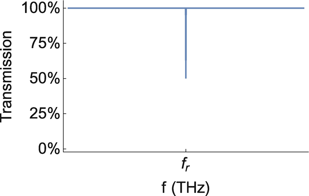
Figure 2:A completely reasonable, but incorrect, guess for the transmission plot. For a transmission plot, 100% means that no photons are absorbed by the atoms, 50% means that half of the photons are absorbed, and 0% means that all of the photons are absorbed by the atoms
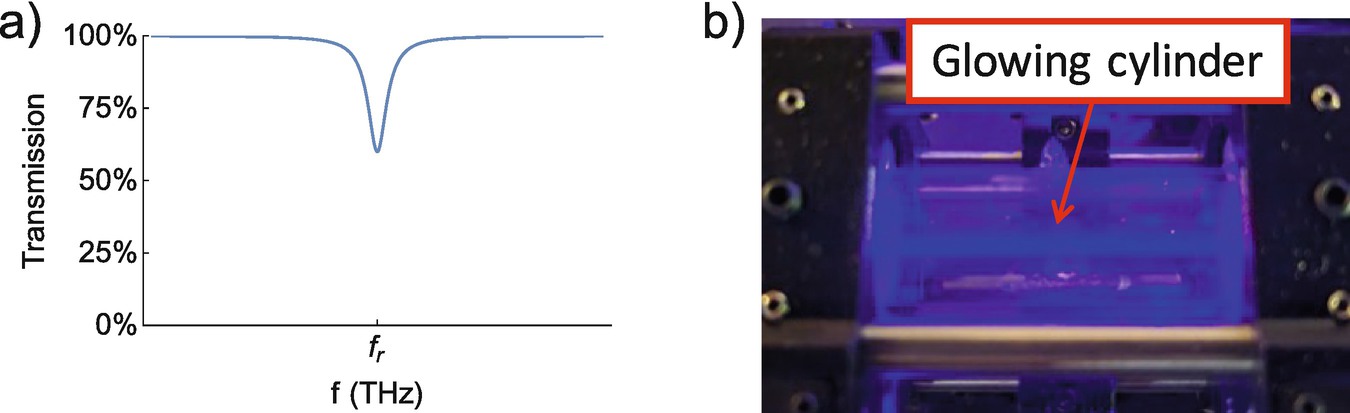
Figure 3:(a) A more accurate transmission plot for the thought experiment. (b) A picture of a laser beam whose frequency matches a resonance frequency near 459 nm (blue light) passing through a vapor cell of cesium atoms. As we scan the laser frequency from below the resonance frequency to above the resonance frequency, we visually see no glowing cylinder, followed by a glowing cylinder (resonance), followed by no glowing cylinder. On resonance, the transmission decreases as shown in (a) because the atoms take photons from the laser and re-emit them in all directions, and almost none of these re-emitted photons continue along their original path to the detector. Note that the transmission plot in (a) is a theory plot assuming that the atoms are at rest. In the vapor cell the atoms are not frozen in place. Chapter 4. Atoms in Motion will explore a transmission plot for atoms moving around
Often times spectroscopists would rather look at an absorption plot instead of a transmission plot, see Fig. Figure 4. An absorption plot is the fraction of photons lost as a function of laser frequency. It looks very similar to a transmission plot, but it has a bump instead of a dip. Both an absorption plot and a transmission plot tell us the same information: atoms absorb (and re-emit) photons from the laser around the resonance frequency. If you add absorption to transmission, you should get 100% for all laser frequencies.
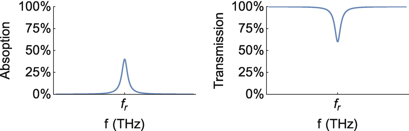
Figure 4:An illustrative example of an absorption plot (left) and a transmission plot (right). If you add these two plots together, you would get 100% for all laser frequencies
The natural linewidth is the full width at half the maximum (FWHM) of the absorption bump, see Fig. Figure 5. It is a property of the transition that we cannot change. As an analogy, think about the charge or mass of an electron. The charge of the electron is simply the charge of the electron, which is . The mass of the electron is simply the mass of the electron, which is . These are intrinsic properties of the electron that we cannot change. The natural linewidth of a transition is inherent for that transition, and we cannot change it.
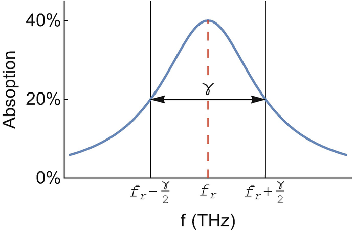
Figure 5:A zoom in of a spectral feature. The natural linewidth is the full width half maximum of this feature
The shape of the bump (or dip in the transmission plot) is often referred to as a spectral feature or spectral profile. For completeness, the width of the spectral feature we measure in the lab is always larger than the natural linewidth because of various “broadening” mechanisms. One of these broadening mechanisms is laser power, which we will discuss in Sect. 3.5 Power Broadening. If the laser power was the only broadening mechanism, we would find that as the laser power gets smaller and smaller, the width gets narrower and narrower until it reaches the natural linewidth. The natural linewidth is the minimum possible FWHM of a spectral feature.
The mathematical shape of the spectral feature is a Lorentzian function. In the absence of any broadening mechanism, the mathematical form is:
where is the natural linewidth[1] and A is the maximum absorption, which describes the amount of laser light lost when traveling through an atomic sample when the laser light is perfectly on resonance. A is a number between 0 (no light absorbed) and 1 (all light absorbed, which is also 100%). You may be familiar with a similarly shaped Gaussian function. A Lorentzian function looks very similar, but it is slightly different in shape.
Math Assessment
Equation (1) is the mathematical shape of a spectral feature. According to Fig. Figure 5 (and the definition of natural linewidth), the absorption at should be half as large as the absorption when . So, let’s check to make sure the formula matches that statement. To do this, we will first plug in into Eq. (1) to make sure that :
Next, we will plug in to see if . If you are more comfortable doing this twice, once for and once for , please do so!
Yay!
Important
Spectroscopists being spectroscopists call the spectral feature many different things. Other common descriptions of the spectral feature include the Lorentzian profile, the absorption profile, the absorption lineshape, the spectral profile, the spectral lineshape, or the Doppler-free spectrum. The description “Doppler-free spectrum” will make more sense after Chap. 5. Saturated Absorption Spectroscopy. Some atomic physicists use the descriptor “Lorentzian function”, but that should be avoided because that phrase is a mathematical definition of that function itself. As an analogy, think about how many times you have used a sine wave or a cosine wave in math. These are mathematical functions that are used to describe lots of different physical phenomena like an oscillating spring or a swinging pendulum. The same thing is true with the Lorentzian function. There are other physical phenomena described by a Lorentzian function, so we instead use more specific language. For the rest of the book, we will use the term spectral feature or spectral profile.
Definitions
Transmission plot: A plot of the percentage or fraction of photons that passes through a vapor cell as a function of laser frequency.
Absorption plot: A plot of the percentage or fraction of photons lost from a laser after it passes through a vapor cell as a function of laser frequency. A dip in a transmission plot is seen as a bump in the absorption plot.
Natural linewidth: The minimum possible full width at half maximum (FWHM) of a spectral feature. The natural linewidth is a property of a transition, with each transition in an atom having a unique natural linewidth.
One Last Thing
We can now update that important statement from Chap. 1. Introduction to Atoms and Light, which is also at the top of this section.
Important Statement
A photon has a probability of being absorbed by an atom depending upon the photon’s energy. It is most likely to be absorbed if the photon’s energy exactly matches the energy difference between the ground and excited state, but there is a non-zero probability of absorption off resonance.
Specifically, in the absence of any broadening mechanism (like laser power), if the photon’s energy is off by from that resonance energy, the photon is half as likely to be absorbed compared to a photon that has the energy equal to the energy difference between the ground and excited states.
3.2 The Natural Linewidth in Angular Units
Many formulas that spectroscopists and atomic physicists use contain variables with angular units. This is more of a mathematical convenience, but since they are used so often, I wanted to introduce them as a topic. Suppose we had a simple sine wave that described an oscillation in time with frequency f and amplitude A. We would write that as:
The presence of in the argument of the sine function stems from the inherent periodicity of a sine wave, which repeats itself every radians. Consequently, each time the argument of the sine function increases by , the waveform completes one full cycle. Thus, the frequency denotes the rate at which the sine wave repeats within a time span of one second. This periodicity of is where the “angular” part comes in. Instead of always writing , we simplify things by using angular frequency, . That curly-looking symbol is the lowercase Greek letter omega. That same sine wave using angular frequency units is:
In the lab, we measure frequency, but, mathematically, we often use angular frequency. The natural linewidth is a frequency, but it is often written in formulas using angular frequency units. In this book, we will use capital gamma, , for the natural width in angular frequency units and lowercase gamma, , for normal frequency units. The relationship between the two is:
I want to emphasize that frequency, and not angular frequency, is the unit that we work with in the lab. To help us keep these two parameters separate, we use the unit radians/second for angular frequency and inverse seconds or hertz (Hz) for frequency. If you are given the information that , then we calculate for use in the lab. If we want to change the frequency of a laser by one linewidth, we change the frequency by , not . Again, to avoid confusion, we don’t use the unit MHz for the angular frequency. Instead, we make sure to use rad/s: .
Reduced Planck’s Constant
In the explanation of the photoelectric effect, Einstein discovered that a photon has an energy . If we wanted to write this equation using angular units, we would get . Physicists absorb that extra into h and call that new constant the “reduced Planck’s constant”: . Notice that the variable for the reduced Planck’s constant resembles a lowercase h with a horizontal line drawn across its stem. We call this constant “h-bar”. We now have two completely equivalent ways of writing the energy of a photon:
It doesn’t matter what equation you use, you will always calculate the same energy.
Any function expressed in frequency units can be written in angular frequency units. For example, the Lorentzian function from Eq. (1) using angular frequency units is:
where is the angular resonance frequency.
3.3 The Natural Linewidth and the Lifetime of the Excited State
The natural linewidth is, remarkably, related to the lifetime of the excited state. To understand the lifetime of an atomic state, first imagine that all of the atoms from the above thought experiment are in the excited state. Next, we turn off the laser beam. As time progresses, the atoms will each emit a photon to go back to the ground state at a random time. Spectroscopists often use the word “decay” when talking about an atom emitting a photon to go back to the ground state. This is a random process, so some atoms decay back to the ground state quickly while others take their time. Statistically, each atom has a probability of decaying out of the excited state that will look like Fig. Figure 6. At , all the atoms are in the excited state. As time marches on, atoms start to decay and the excited state fraction gets smaller. For the graph in Fig. Figure 6, about 63% of the atoms have decayed back to the ground state in 6.25 ns, and about 80% of the atoms have decayed back to the ground state in 10 ns. The mathematical form of the decay curve is:
where (this is the Greek letter lowercase tau) is called the lifetime of the excited state. This function is called an exponential decay. Like the natural linewidth of a transition, has a unique value for every transition in an atom. The lifetime of the excited state used for the decay in the graph is , which means that after about 63% of the atoms have decayed. There is nothing special about 63%; it is just what physicists decided to define as the lifetime. Mathematically it is a nice definition because when , the fraction of atoms that have not decayed is , or 36.8%. After two lifetimes , about 86.5% of the atoms have decayed leaving , or 13.5%, of the atoms in the excited state.
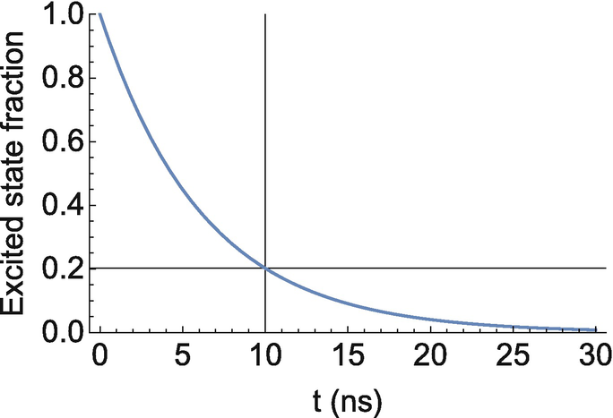
Figure 6:The excited state fraction as a function of time for an excited state that has a lifetime of 6.25 ns
Amazingly, the natural linewidth and the lifetime are related! The formula relating the two quantities is:
As you can imagine, atomic physicists and spectroscopists often use the angular frequency form of natural linewidth when thinking about lifetime.[2] These two quantities are inversely related to each other. This means:
If the lifetime is small, the natural linewidth is large. This means that excited states with a small lifetime have absorption and transmission plot spectral features that are relatively wide.
If the lifetime is large, the natural linewidth is small. This means that excited states with a large lifetime have absorption and transmission plot spectral features that are relatively narrow.
3.4 The Scattering Rate and Saturation
Definitions
Waist of a laser: The half width of the intensity plot where the intensity is 13.5% of the maximum intensity, see Fig. Figure 7. We use the variable w to represent waist.
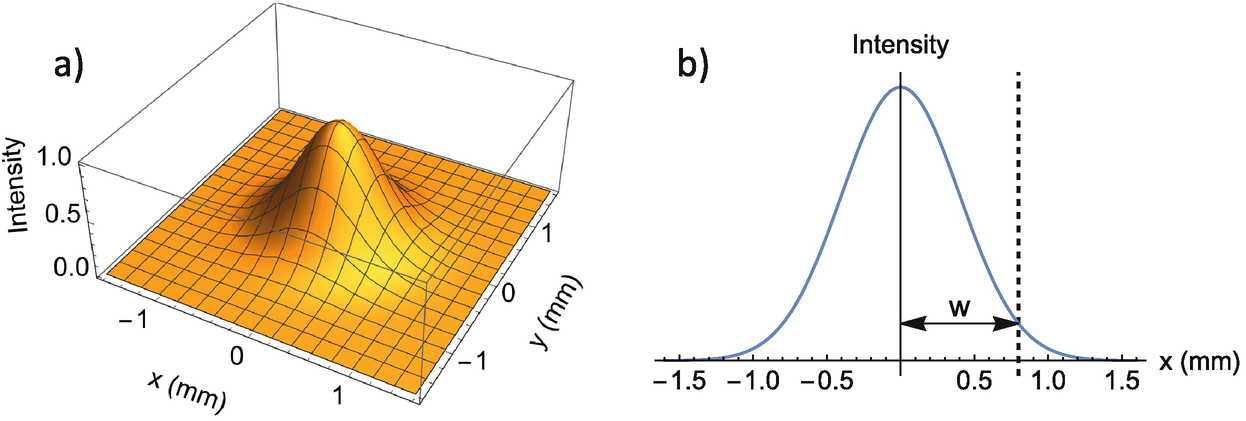
Figure 7:(a) The intensity of a laser beam on the wall. (b) The intensity along any one of the axes. The waist is the half width of the intensity plot when the intensity is 13.5% of the maximum intensity
Intensity: The intensity of a laser beam is the power of the laser divided by the cross sectional area of the laser beam, denoted as .
If you shine a laser on the wall, you will see something that appears to be a circle. However, it isn’t actually a circle. If we plotted the intensity of the laser, it would look like Fig. Figure 7a. The waist of a laser beam is defined in Fig. Figure 7b. It is a bit confusing since most people think of the waist of a laser as the diameter, but it is more similar to a radius. The intensity profile is described by a Gaussian function.[3] The area of a laser beam is:
This is, of course, for a perfect laser beam. In real life, the intensity profile is not a perfect Gaussian function and the waist in the x direction and y directions could be different. In the latter case, the cross sectional area of a laser is
Guiding Question:
We are interested in the following question: Given a laser and a particular transition in an element, how many photons per second will that atom absorb (and re-emit)? This value is known as the scattering rate. Take a few moments to think about this question before continuing.
Intensity Versus Power In the lab, we measure laser power. However, we actually care about laser intensity. Why? (This is a homework problem as well).
How many photons an atom scatters depends upon a few different ideas: (1) how far the laser frequency is from the resonance frequency relative to the natural linewidth, (2) how long an atom spends in an excited state, and (3) how a transition reacts to photons from a laser whose frequency matches the resonance frequency. Let’s unpack all of these ideas.
We now know that the shape of the absorption bump has the mathematical form of a Lorenztian function. For spectroscopists, the natural linewidth really matters. Suppose an atom has a natural linewidth of and the laser is below the resonance frequency, see the left spectral profile in Fig. Figure 8. For this transition, the atom will “scatter” (i.e., absorb and re-emit) many photons from the laser. The right spectral profile in Fig. Figure 8 corresponds to a transition that has a natural linewidth of . For this narrower transition, the atom will not scatter many photons at all even though the laser frequency is still set to below the resonance frequency.
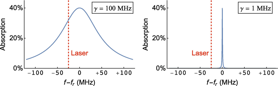
Figure 8:Two examples for how light from a laser interacts with two different transitions. The left transition has a large natural linewidth while the right transition has a small natural linewidth. The laser frequency (red dashed line) is 25 MHz below the resonance frequency for both transitions
To quantify how far the laser frequency is from the resonance frequency, we define a new parameter called detuning. Detuning, which is represented by the lowercase Greek letter delta in normal frequency units and capital delta for angular frequency units, gives us this information. Mathematically, detuning is , where f is the frequency of the laser. Notice that if , then . In the lab, we call this “red detuning,” which will make more sense after we discuss the Doppler effect in Chap. 4. Atoms in Motion. Likewise, if , then , which we call “blue detuning.” In our thought experiment, the atoms will absorb the largest number of photons when (the laser frequency exactly matches the resonance frequency). In the absence of power broadening (i.e., when the laser power is kept low), the atoms will absorb half as many photons when or compared to when .
As discussed above and displayed in Fig. Figure 8, detuning is important, but so is the natural linewidth. What we really want to know is how far the laser frequency is from the resonance frequency relative to the natural linewidth. For example, if we set the laser frequency such that , the laser will lose half as many photons compared to when . This is true for any transition. The quantity that matters for the scattering rate is the ratio of detuning to natural linewidth. So, we expect to show up in the relevant scattering rate equation.
The scattering rate tells us how many photons are absorbed (and re-emitted) by an atom. From point (1), we know that detuning matters. The average time an atom spends in the excited state also matters. If an atom, on average, spends only 1 ns in the excited state, it decays very quickly, freeing itself up to be excited again. Contrast that with an atom that spends, on average, 2 seconds in the excited state. That atom will have a very small scattering rate. From Eq. (10), we know that the average lifetime is related to the natural linewidth. A large natural linewidth means a short lifetime. Therefore, a large natural linewidth results in a large scattering rate.
Let’s consider two transitions with different resonance frequencies. Transition #1 has a resonance frequency and transition #2 has a resonance frequency . We will assume that and that both transitions have the same natural linewidth. We also have two lasers with the same intensity. The frequency of laser #1 is set to and is sent through a vapor cell with atoms that have transition #1. The frequency of laser #2 is set to and is sent through a vapor cell with atoms that have transition #2. In other words, the only difference between the two experiments is that transitions have different resonance frequencies. Will both transitions scatter (i.e., absorb and re-emit) the same number of photons per second, or will the scattering rates be different?
Surprisingly, the answer is that the scattering rates are different for the two transitions! The reason is that the cross section (or “size”) of the photons is different for the two transitions. Roughly, the cross section of a photon is . If a transition has a smaller resonance frequency, the laser light has a longer wavelength and photons with a bigger cross section. That means the photons in the laser are “big” and more likely to “hit” the atom and cause the transition. If a photon has a small cross section (high frequency, short wavelength), it is less likely to hit the atom and cause the transition. For the example above, the photons from the laser with have a smaller cross section than the photons from the laser with . If we want the same number of scattered photons from the two transitions, the atom with needs to be exposed to more photons than the transition with . In other words, to achieve the same scattering rate for the two transitions, the transition with requires a higher intensity than the transition with .
Summary
Detuning relative to the natural linewidth matters. should have the largest scattering rate.
The natural linewidth (or lifetime of an excited state) matters. Large should have a large scattering rate.
Photon cross section matters. A large frequency, or short wavelength, has a smaller scattering rate.
To quantify points (2) and (3), we introduce a parameter known as the saturation intensity . The saturation intensity contains all the information about a particular transition that helps us understand how easily an atom interacts with photons in a laser beam whose frequency matches the resonance frequency of a transition (we will quantify this statement soon). Suppose we send a laser beam whose frequency matches the resonance frequency for some transition through a sample of atoms. If an atom absorbs a photon, it will spend some amount of time in the excited state before decaying back to the ground state, where it is free to absorb another photon. The saturation intensity is the laser intensity for an on-resonance laser () such that 25% of the atoms are in the excited state at any given time. A transition with a small saturation intensity means that we only need a small laser intensity to have 25% of the atoms in the excited state. A transition with a large saturation intensity means we need a large laser intensity to make that happen.
The ratio of the intensity of light to the saturation intensity is called the saturation parameter . We like to use s because, like , it means the same thing for every transition. Saying means that we set the laser intensity equal to the saturation intensity. Some transitions might have a high saturation intensity, like a transition in the beryllium atom that has , while other transitions have a low saturation intensity, like a transition in the cesium atom that has . For that transition in the beryllium atom, we would need of power for a laser with cross sectional area to have , which means 25% of the atoms are in the excited state. 885 mW is a lot of laser power! For the transition in the cesium atom, we only need of power to have 25% of atoms in the excited state. The formula for the saturation intensity is:[4]
Notice that the saturation intensity is proportional to . This is point (2). Also notice that there is a in the denominator. One of those terms is grouped with hc in the numerator; represents the energy of the on-resonance photon. The remaining comes from the cross section of a photon. The saturation intensity is a property of a transition! It is whatever it is, and it cannot be changed.
Assessing the Scattering Rate Formula Before We Even Write It Down
Before we write down the formula that models the scatter rate, decide if should be in the numerator or the denominator? In other words, would result in more or less photons scattered compared to ? What about the saturation parameter s? Should that parameter be in the numerator or denominator?
The scattering rate, which is derived using quantum mechanics, is how many photons per second an atom will absorb (and re-emit). The scattering rate, using angular frequency variables and using normal frequency variables, is:
The equation using normal frequency units is more practical, but you will rarely see that formula written anywhere. Almost every atomic physics textbook will use the scattering rate formula that uses angular frequency variables. Notice that the ratio is in the denominator. If that number gets big, the scattering rate decreases. The saturation parameter is in the numerator and the denominator, which you might not have guessed. It makes sense for it to be in the numerator because if I increased the laser intensity there are more photons for the atom to interact with making it more likely to absorb and emit a photon. But what about the extra s in the denominator?
The first thing to notice is that if the saturation parameter is small, than , and s would only be in the numerator. The extra s in the denominator comes from the fact an atom will always spend some amount of time in the excited state. If we got rid of the s in the denominator, the number of photons scattered per second (i.e., the scattering rate) is linear with laser power. That means if we increase the laser power by some factor, we increase the scattering rate by the same factor. However, the atom spends, on average, time in the excited state. If the atom is already in the excited state, it can’t absorb a photon. If all the atoms were in the excited state, there are no atoms left in the ground state to absorb any photons.
This is important, so let’s explore it a little more. Suppose an atom always spends a time in the excited state before decaying back to the ground state.[5] In the most extreme case of super high laser intensity, an atom would be immediately re-excited back to the excited state before having to wait another 10 ns to decay. In this most extreme case, the atom can only absorb 1 photon every . That means, at most, an atom can absorb photons every second. Without the s in the denominator, the scattering rate would increase without bound as the power increases. However, with the s in the denominator, the on-resonance scattering rate will “saturate” at .[6]
Summary of Formulas
One Final Thing:
The fraction of atoms in an excited state was one of the key concepts we used to explore the scattering rate. So, it is no surprise that scattering rate also tells us what fraction of atoms are in the excited state. The fraction of atoms in the excited state is (use the angular frequency formulas for calculating the excited state fraction).
Let’s do a quick assessment. If (or ) and , the excited state fraction should be 25%:
3.5 Power Broadening
The scattering rate tells us how many photons per second an atom takes from the laser. A large scattering rate must correspond to a larger amplitude spectral feature in an absorption plot. In fact, atoms scattering photons is the only way to produce a spectral feature. If that is the case, shouldn’t the scattering rate be a Lorentzian function (Eq. (1)) like our spectral features? It looks close, but there is that extra s in the denominator of the scattering rate that is not in Eq. (1). While it might not look like it, the scattering rate is a Lorentzian function. We just need to do a little algebra to convert the scattering rate into a new form. The algebraic step is to factor out from the denominator:
We are going to define a new parameter , known as the power broadened linewidth. With this definition, we can write as . To help us assess this formula, we will also switch the positions of s and in the numerator. With those changes, we have:
This is now a Lorentzian function with amplitude and FWHM of . As we increase the saturation parameter s (i.e., increase the laser intensity), the FWHM of the scattering rate becomes larger by a factor of . Therefore, the width of a spectral feature increases by the same amount. Also notice that when , the FWHM reaches its minimum value of the natural linewidth.
Next, let’s analyse the amplitude. As the saturation parameter gets larger and larger, , so . The amplitude saturates! As the laser power increases, the amplitude approaches the maximum scattering rate of . However, the FWHM never saturates; it continues to broaden, as shown in Fig. Figure 9.
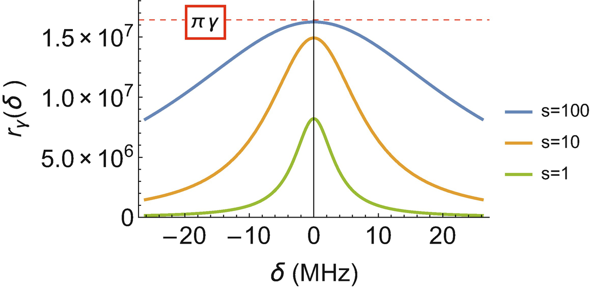
Figure 9:The scattering rate for a transition with as a function of detuning for different saturation parameters. The red dashed line is the maximum possible scattering rate
Finally, let’s put some numbers in to start getting comfortable with real scattering rate numbers. For the example in Fig. Figure 9, I used the natural linewidth for a transition in the cesium atom near 852 nm. The natural linewdith is about . The on-resonance scattering rate is 8.2 million photons absorbed (and re-emitted) per second for ; 14.9 million photons per second for ; 16.2 million photons per second . For a typical transition, scattering hundreds of thousands to millions of photons per second is not unusual. Notice that when s is small, the scattering rate at is almost 0; mathematically, it is about 270,000 photons/sec for . However, the scattering rate for remains quite sizable.
For completeness, there are other factors that can broaden the width of a transition including temperature (this is the topic of Chap. 4. Atoms in Motion) and pressure. We do not cover pressure broadening, also known as collisional broadening, in this book.
3.6 Example
A lot has happened in this chapter, but two of the important concepts are that (1) the scattering rate tells us how many photons per second an atom absorbs (and emits) from the laser and (2) the cumulative effect of all the atoms taking photons results in the absorption profile. Let’s solidify these concepts with an example. Throughout this example, we will also introduce some commonly used language in atomic physics. A lot of the language will be explored in more detail as we work our way through this book.
A particular type of barium atom[7] called barium-135 has one ground state and three closely spaced excited states, see Fig. Figure 10. The spacing between the excited states is called hyperfine splitting, which will be explored in detail in Chap. 9. Hyperfine Structure. The reason there are three excited hyperfine states is because the nucleus has angular momentum, a concept we will begin exploring in Chap. 7. Angular Momentum. If the nucleus did not have angular momentum, there would be only one excited state.[8] Again, we will learn the physics behind hyperfine splitting starting in Chap. 7. Angular Momentum. Before we do an example, we need a few more definitions.
![A simplified Grotrian diagram for a transition in the atom known as barium-135. The energy spacings are not to scale. The energy spacings between the excited hyperfine levels are calculated from the results of Baird et al.[1]. The center of gravity frequency is extracted using numbers from both Baird et al. [1] and Karlsson et al. [2]. The uncertainty in the center of gravity frequency is about 30 MHz. [2] While that isn’t a terrible uncertainty, modern day spectroscopic methods can do better!](/AtomicPhysicsForEveryone/build/541577_1_En_3_Fig10_-e3abefa19d8c642d2500297012d8b668.png)
Figure 10:A simplified Grotrian diagram for a transition in the atom known as barium-135. The energy spacings are not to scale. The energy spacings between the excited hyperfine levels are calculated from the results of Baird et al.[1]. The center of gravity frequency is extracted using numbers from both Baird et al. [1] and Karlsson et al. [2]. The uncertainty in the center of gravity frequency is about 30 MHz. [2] While that isn’t a terrible uncertainty, modern day spectroscopic methods can do better!
Definitions
Center of gravity: The energy of a state if the nucleus had no angular momentum.
Hyperfine splitting: When the nucleus has angular momentum, the single energy level at the center of gravity splits into multiple energy states. Each of these states is going to shift in energy a small amount compared to the center of gravity energy.
Bra-ket notation: Atomic physicists sometimes use “bra-ket” notation when working with states in an atom. A “ket” is a way to represent a particular state and it looks like this: . A “bra”, which is not used in this book but you will use it a lot if you take quantum mechanics, looks like this: . Bra-ket notation is also referred to as Dirac notation, named after the English mathematical and theoretical physicist Paul Dirac.
Note
Some learners may use only Part 1 of this book. I wanted to introduce you to bra-ket notation so that you have seen it at least once before you take quantum mechanics. We are going to use it in this example and in Problem Exercise 3.9, but it will not be used again until Part 2. You are, of course, welcome to use bra-ket notation if you want, but it is not necessary. You may also see bra-ket notation if you take a linear algebra class.
As seen in Fig. Figure 10, we are going to label the ground state and the three excited states , , and . F is called a quantum number, and it is always a positive integer, a half integer, or zero; quantum numbers are explored starting in Chap. 6. Quantum Mechanics vs. Classical Physics. For now, these quantum numbers are just being used to label our states. Notice there is a center of gravity frequency, , that tells us the energy difference between the center of gravity for the two states. This tells us that our transitions are all around 541.4 THz, or 553.7 nm. Each hyperfine level is shifted from their center of gravity state by a small amount. I want to emphasize that if a nucleus has angular momentum, the center of gravity states do not exist in real life! The hyperfine states are the actual states. However, we can learn a lot of physics by determining how the hyperfine levels shift from the center of gravity, which is explored in Chaps. 9. Hyperfine Structure and 10. Isotope Shifts, Radioactive Decay, and the Nuclear Forces.
3.7 Problems
References
Baird, P.E.G., Brambley, R.J., Burnett, K., Stacey, D.N., Warrington, D.M., Woodgate, G.K.: Optical isotope shifts and hyperfine structure in 553.5 nm of barium, Proc. R. Soc. Lond. A365567–365582 (1979). Baird et al. (1979)
Karlsson, H., Litzén, U.: Revised Ba I and Ba II wavelengths and energy levels derived by fourier transform spectroscopy. Phys. Scripta 60, 321 (1999). Karlsson & Litzén (1999)
Thibault, C., Touchard, F., Büttgenbach, S., Klapisch, R., de Saint Simon, M., Duong, H.T., Jacquinot, P., Juncar, P., Liberman, S., Pillet, P., Pinard, J., Vialle, J.L., Pesnelle, A., Huber, G.: Hyperfine structure and isotope shift of the line of 76–98Rb and some of their isomers. Phys. Rev. C 23, 2720 (1981). Thibault et al. (1981)
This is for the low power limit. In Sect. 3.5 Power Broadening, we will refine this formula slightly to include power broadening. I just want to start basic to get the concepts first.
A careful reader might notice the units for lifetime look like . You can think of radians as simply a placeholder to remind us to use radians () instead of degrees () in our math when calculating frequency. We do not keep the radian unit for lifetime. That unit for lifetime is seconds (or \upmu \text{s} or ns).
A Gaussian function is very similar to a Lorentzian but it is slightly different. We will explore Gaussian functions more in Chap. 4.4 The Maxwell-Boltzmann Velocity Distribution.
For completeness, this is the formula for doing spectroscopy with linearly polarized laser light. Experiments with circular polarized light have a slightly different formula.
Remember that an atom actually decays probabilistically with a characteristic time . This is just a thought experiment to understand the concept of saturation.
A careful reader might notice the maximum scattering rate is only half as big as our thought experiment predicted. The idea of the thought experiment is correct, but we are ignoring an effect known as coherent state transfer, which includes stimulated absorption and stimulated emission. This is a massive, complicated topic, and one that is beyond the scope of this book. In fact, most quantum mechanics classes don’t get to this idea until the very end of the semester, if they get to it at all. Including this extra physics reduces the maximum scattering rate by a factor of 2.
All barium atoms have 56 protons in the nucleus. Neutron number can vary from about 58–97! We call a particular barium atom, for example an atom with 56 protons and 79 neutrons, an isotope of barium. Isotopes are explored in Chap. 10. Isotope Shifts, Radioactive Decay, and the Nuclear Forces.
There are atoms with ground state hyperfine splitting; barium-135 is just not one of those atoms.
We only need this rule for the moment. A full list of the rules that need to be satisfied for an electron to transition between two atomic states is given in Appendix C.
- Baird, P. E. G., Brambley, R. J., Burnett, K., Stacey, D. N., Warrington, D. M., & Woodgate, G. K. (1979). Optical isotope shifts and hyperfine structure in ⋋553.5 nm of barium. Proceedings of the Royal Society of London. A. Mathematical and Physical Sciences, 365(1723), 567–582. 10.1098/rspa.1979.0035
- Karlsson, H., & Litzén, U. (1999). Revised Ba I and Ba II Wavelengths and Energy Levels Derived by Fourier Transform Spectroscopy. Physica Scripta, 60(4), 321–328. 10.1238/physica.regular.060a00321
- Thibault, C., Touchard, F., Büttgenbach, S., Klapisch, R., de Saint Simon, M., Duong, H. T., Jacquinot, P., Juncar, P., Liberman, S., Pillet, P., Pinard, J., Vialle, J. L., Pesnelle, A., & Huber, G. (1981). Hyperfine structure and isotope shift of the<mml:math xmlns:mml=“http://www.w3.org/1998/Math/MathML">http://www.w3.org/1998/Math/MathML” display=“inline”><mml:mrow><mml:msub><mml:mrow><mml:mi>D</mml:mi></mml:mrow><mml:mrow><mml:mn>2</mml:mn></mml:mrow></mml:msub></mml:mrow></mml:math>line of<mml:math xmlns:mml=“http://www.w3.org/1998/Math/MathML” display=“inline”><mml:mrow><mml:mmultiscripts><mml:mrow><mml:mi mathvariant=“normal”>Rb</mml:mi></mml:mrow><mml:mprescripts/><mml:mrow/><mml:mrow><mml:mn>7</mml:mn><mml:mn>6</mml:mn><mml:mo>−</mml:mo><mml:mn>9</mml:mn><mml:mn>8</mml:mn></mml:mrow><mml:mrow/><mml:mrow/></mml:mmultiscripts></mml:mrow></mml:math>and some of their isomers. Physical Review C, 23(6), 2720–2729. 10.1103/physrevc.23.2720