Abstract
In this chapter, we explore angular momentum, a key concept in quantum mechanics and atomic physics. We cover the quantization of angular momentum, the role of quantum numbers, and their impact on atomic states. We will learn about the different types of angular momentum, the states representing these types of angular momentum, and how angular momenta are added together in quantum mechanics. The chapter also examines the compatibility of different observables, such as the magnitude and components of angular momentum, and the impact of measurements on quantum states.
Keywords: Quantum numbers, Angular momentum, Orbital angular momentum, Magnitude projection, Spin, Intrinsic angular momentum, Electronic angular momentum, Adding quantum mechanical angular momentum, Fine structure, Fine structure splitting
Learning Goals
By the end of this chapter, you should be able to understand:
that angular momentum is a vector that has both magnitude and direction.
that quantum mechanics restricts angular momentum to certain discrete magnitudes and directions.
that there are multiple angular momentum vectors in an atom, and understanding how these vectors add together impacts the energy of a particular state.
that quantum numbers are key tools for understanding angular momentum in quantum mechanics.
the concept of compatible and incompatible observables in the context of angular momentum measurements.
7.1 Definitions
Note
There are a lot of new definitions in this section. We will talk about and try to understand all of them, but don’t worry too much about memorizing everything right now. We will use some of the definitions continually throughout the rest of the book. In future discussions, you should come back to these definitions as needed. We are all learners, and learning takes repetition.☺
Momentum
This is the same definition from Chap. 6. Quantum Mechanics vs. Classical Physics: a property of an object that is moving. For a classical object like a baseball, the formula for momentum is , where p is the object’s momentum, m is the object’s mass, and v is the object’s velocity. An object’s momentum will change if something acts on the object from the outside. The larger an object’s momentum, the harder it is to stop. The unit of momentum is .
Force
Below are two definitions of force. The first is the most common definition. However, it is only true if the object’s mass is not changing, which is a very common scenario. The second is the real definition of force. The unit of force is , which we also call a newton (N).
Definition #1
An external interaction that causes an object to accelerate (i.e., change velocity). Imagine pushing a block up a ramp. You are pushing on the block and causing its velocity to change. That push is an external interaction (force) on the block. Any single force acting on an object will cause the object to accelerate (change velocity). There can be multiple forces acting on an object. Sometimes those forces cancel each other out. If there are multiple forces that perfectly balance one another so the net force is 0, then the object will not accelerate. However, if the net force is not 0, it will accelerate. This is summarized by Newton’s 2nd Law: “The sum of all forces acting on an object causes an object with mass to accelerate.”
Definition #2
An external interaction that causes an object’s momentum to change. Newton’s 2nd Law for momentum: “The sum of all forces acting on an object causes an object’s momentum to change.”
Torque
A measure of how effective a force is in causing an object to rotate. The two things that matter for torque are the size of the force that causes the rotation and how far from the axis of rotation that force is being applied. Imagine you have a bicycle wheel. If you exert a force horizontally at the edge of the wheel, the wheel starts to spin. Since that force caused a rotation, there is a torque. Applying that same force on the axle or pushing on the tire directly towards the axle does not cause any rotation, so in those two scenarios there is no torque. The unit for torque is . Interestingly, torque and energy share the same unit: . However, torque is not energy; they are incredibly different!! To avoid confusion, we tend to not write the unit for either energy or torque. We use joules (J) for energy and newton meters (Nm) for torque. Torque will be important in this chapter.
Angular Momentum
A property of an object that is rotating. It is the thing that changes when a torque is applied to the object. There is a parallel between the ideas of force and momentum, and torque and angular momentum. Momentum is a property of an object that is moving along a straight line, and it changes when a force is applied to the object. The larger an object’s momentum, the harder it is to stop the object from moving (a bigger force is needed). In the same way, angular momentum is a property of an object that is rotating, and the object will start to rotate faster or slower when a torque is applied (a bigger torque makes the change happen faster). The unit of angular momentum is . Angular momentum is extremely important in quantum mechanics and atomic physics.
Reduced Planck’s Constant (h-Bar)
.
Important Comment
Both Planck’s constant and the reduced Planck’s constant have units of angular momentum, , which can also be written as joules times seconds, . The reduced Planck’s constant will be used a lot in this chapter. You will see why we call it a fundamental constant.
Quantum Number
In quantum mechanics, a lot of different properties are quantized, i.e., can only have certain values. We already know that the energy levels of an atom are quantized. Other properties, like angular momentum, are also quantized. When something is quantized, a quantum number is usually associated with that property. A quantum number is an integer or half-integer. Knowing a quantum number will allow someone to calculate some property of an atom. Quantum numbers have no units.
As an example, we will soon talk about the electronic orbital angular momentum quantum number (that is a mouthful!). That quantum number is represented by a script . is a quantum number that can be zero or a positive integer: 0, 1, 2, 3, etc. is a discrete number because, according to quantum mechanics, the size or magnitude of the orbital angular momentum of electron is found to have only certain, discrete values. If I tell you that a state in an atom has , we can calculate the magnitude of the electron’s orbital angular momentum. is not the actual size of the orbital angular momentum, but the quantum number can be used to calculate it from the formula . Notice that everything in that formula is either the quantum number or the reduced Planck’s constant. In a way, knowing a quantum number is very similar to how spectroscopists use as an energy unit. is not the correct unit for energy, but we can multiply it by fundamental constants to get the actual energy. The same is true with quantum numbers. Knowing a quantum number is equivalent to knowing a specific property. You might have to do some math, but the only other parameters in the equation should be fundamental constants. So, being told is the same thing as being told that the magnitude of the electron’s orbital angular momentum is . We will soon find that we need many quantum numbers to describe a particular state in an atom.
7.2 Angular Momentum
Electrons, protons, and neutrons all have angular momentum. A classical analogy is thinking about the moon orbiting the earth.[1] The moon has orbital angular momentum because it is orbiting the earth. The moon is also spinning on its own axis, so it also has “spin” angular momentum. So, the moon has two types of angular momentum: orbital and spin. Likewise, an electron in an atom can have orbital angular momentum and spin, which is sometimes called intrinsic angular momentum. Interestingly, an electron always has intrinsic angular momentum, but it does not always have orbital angular momentum. One of the craziest things about quantum mechanics is that we don’t have a great analogy to think about the orbital angular momentum or spin of the electron. The electron is not orbiting around the nucleus or spinning on its axis like the moon, but it has the same properties as if it were. The electron, as far as we can tell, has no size! So, how can it be spinning? Imagine how confusing that must have been when physicists were first trying to understand the electron.[2] It has all the properties one would expect for a ball spinning on its axis, but it is not a ball and it is not spinning! Understanding electron spin is still a wonderful mystery.
Since there are two types of angular momentum, we could ask the question, “What is the total electronic angular momentum of the electron in an atom?” The total electronic angular momentum is not a simple sum of orbital angular momentum and spin. In other words, you cannot just add the two angular momenta together like . Angular momentum is something called a vector, which is something with magnitude (i.e., size or length) and direction. To get the total electronic angular momentum you have to add the orbital angular momentum and spin together in their vector forms. As a classical analogy, imagine you walk 30 m due north, see Fig. Figure 1. That is a vector because it has a magnitude (30 m) and a direction (due north). Next, you walk 40 m due west. Once again, that is a vector. If you were to add the two vectors together, you would be asking the question, “If I restarted my journey but took the shortest path, how far and in what direction would I walk?” The answer to this particular scenario is 50 m at West of North.
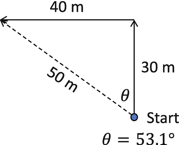
Figure 1:An example of adding two vectors together
The Super Important Take Home Message
Adding two vectors together produces a third vector. The size and direction of the third vector depends upon the sizes and directions of the first two vectors.
Let’s get back to talking about angular momentum in a quantum system. An electron in an atom has a total angular momentum. That total angular momentum of the electron comes from the vector addition of its orbital angular momentum and its spin. There are quantum numbers associated with all three of these angular momentum vectors (orbital, spin, and total). The rest of this chapter is going to be focused on understanding angular momentum in a quantum system. We will find that both the size and direction of an angular momentum vector are quantized (i.e., can only have certain values like the size of an orbital angular momentum vector is where is a positive integer or zero). We will start by exploring the orbital angular momentum of a single electron in an atom and then build up the complexity by exploring (and adding) more and more angular momentum vectors to the system.
7.3 Orbital Angular Momentum of a Single Electron
The magnitude of the orbital angular momentum vector for a single electron in an atom is represented by the quantum number . The direction (or orientation) is also quantized and is represented by the quantum number . Fig. Figure 2a) shows an example of the three possible orientations of an orbital angular momentum vector represented by . Each of these vectors has the same magnitude (they all have ), but they all point in different directions (they all have a different quantum number). While tells us the magnitude of the vector, tells us how much of the vector points along the z-axis; this is called the z-component or z-projection. Fig. Figure 2a) has three values of : 1, 0, and +1. The dashed blue circles are meant to indicate that the angular momentum vector points anywhere on that circle. Because the angular momentum vector can point anywhere on the circle, some people like to think of angular momentum as a cone, see Fig. Figure 2b).[3] These cones are also referred to as angular momentum states, which we will make more sense as we work our way through Chaps. 7. Angular Momentum and 8. Electronic Structure and Atomic Notation.
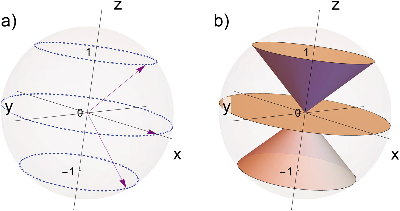
Figure 2:Two popular ways to think about angular momentum states for a quantum mechanical system, like an electron in an atom. (a) A vector representation of the three possible vector orientations for an electron with orbital angular momentum quantum number . (b) The same information using cones instead of a vector and a dotted circle
Orientation of the angular momentum vector, height of the cone, or component/projection along the z-axis are all valid ways to think about . After solving the math for quantum mechanics, we find the component of orbital angular momentum along the z-axis to be . For the upside-down cone in Fig. Figure 2b), the orbital angular momentum vector is represented by the two quantum numbers and , or the size of the orbital angular momentum is and the amount of orbital angular momentum along the z-axis (or height of the cone) is . The flat cone has the same size (), but it has no component along the z-axis (). Finally the upright cone has a component along the z-axis represented by . Since is the amount pointing along the z-axis, that number is also restricted by the value of . For example, if , cannot be 2. If it was, the amount pointing along the z-axis would be larger than the total magnitude!
Experimentalists can measure these values. If an electron in an atom has orbital angular momentum represented by , the experimentalist will measure the size to be every single time. However, if they measured the z-component, they could find , 0, or . But wait, couldn’t they measure the x-component? What makes the z-component quantized while the x- and y- components just have to be somewhere along the dashed blue circle? On that note, how does an electron even decide which direction is z?
The general answer to all those questions is that we (the physicists) just decided to call one of the directions z. After we randomly pick a direction and call it z, we measure the amount along that axis. When we do that, we will only find those three values: , 0, or . We could certainly measure the x-component and get a value. In fact, if we measured the x-component we would get three possible values: , 0, or . The pictures in Fig. Figure 2 would look very similar except the circles/cones would be aligned along the x-axis. Let’s call those components , , and . The three possible values for the z-component form a basis set of size three. The three possible values for the x-component also form a basis set of size three, but those states making up that basis set are different than the state making up the basis set for the z-component. More importantly, those two basis sets are incompatible with each other.
Reminder of Important Definitions
Incompatible observables: If two observables cannot be precisely measured at the same time, they are called incompatible. Measuring one observable changes the system, making subsequent measurements of the other observable unpredictable.
Compatible observables: If two observables can be precisely measured at the same time, they are called compatible. Measuring one observable does not change the system in a way that affects the measurement of the other observable. Remeasuring the first observable will return the same value as initially measured.
Important
In the following paragraphs, all of the states are for angular momentum. I am going to use to represent the z-component of the angular momentum state, for the y-component, and for the x-component.
Suppose our system is in a state . This is the upright cone in Fig. Figure 2b). Since the x- and z- components are incompatible, we don’t know what we will measure along the x-direction. We know there will be three possible outcomes for the amount of angular momentum along the x-axis (, 0, or ), but we don’t know which value we will find until we measure it. This concept is what is being represented by the blue circles or the cones.
Mathematically, we can also think about this using the principle of superposition. Each set of three cones forms a basis set. One basis set is the three cones representing orbital angular momentum along z and other is the three cones along x. A state from one basis set can be constructed from a superposition of the other basis set. For example,
where is the state representing that upright cone (orbital angular momentum along z), , , are the three states making up the x-component of the orbital angular momentum basis set, and , , and are the probabilities that, upon measurement of the x-component of angular momentum, the system has x-component values , , or (remember the actual value of the x-component of orbital angular momentum is ). We could repeat the same argument with the y-component. In fact, all three components are incompatible with each other. To summarize this, here are the three basis sets:
Each state represents a cone along a particular axis. We are certainly allowed to measure any component of angular momentum we want. Upon measurement, we will be in one of those states. However, since they are all incompatible observables, measuring one of the components puts the system in a superposition of the states for the other obervables. Interestingly, we have two separate ways to construct the state :
In a way, this makes sense. If the quantum mechanical system is in the state and we measure the x-component of angular momentum, we will get with probability , with probability , or with probability . On the other hand, we could have decided to measure the y-component at which point we would need to construct the state from the y-basis set to predict what we would measure if we measured the y-component. I should point out that we can calculate those amplitudes using quantum mechanics. For this particular system, , , and .
Ok, so all three components are incompatible with each other, but what about compatibility with the magnitude of the angular momentum vector? Interestingly, the magnitude of the angular momentum vector is a compatible observable with all three components of angular momentum! At first, this might seem a little weird; how can all the components be incompatible with each other yet each component is compatible with the magnitude? But, in a way, this also makes physical sense. The length of the vector is the same whether the cones point along the x-direction, the y-direction, or the z-direction. Measuring a component of angular momentum does not change the length, but it does change the orientation. For this system, measuring the magnitude of angular momentum will always return (or ). It doesn’t matter if we are in a state for the x-component, y-component, or z-component, .
The rest of the chapter will be spent making the system more complex and complete. To do this, we will need to pick one component of angular momentum to represent the system. Since the x-, y-, and z- components are just rotations of each other, it doesn’t really matter which one we use to represent direction. By tradition, we pick the z-component.
In the end, the above discussion can be summarized as follows: for , there are three possible projections for an axis and they all look the same (, 0, and ). So, we need to pick some axis to represent the idea that there are three orientations for the orbital angular momentum vector.
A lot has happened in this section, so let’s summarize:
Summary
Orbital angular momentum is quantized in two ways: the magnitude and the projection on an axis.
The magnitude is represented by the quantum number , which is used to calculate the magnitude using the formula .
The component of the orbital angular momentum along the z-axis is represented by the quantum number , which is used to calculate the component along the z-axis using the formula .
The choice of the z-axis is random, but we need an axis to represent the fact that there are only certain directions the vector can point along that axis.
We can still measure along other directions, but the measurements along those directions are incompatible with measurements along the z-direction. We use cones to remind us that, while we know the z-component of angular moment, the x- and y-components are incompatible with the z-component.
7.4 The Magnitude and Projection of Angular Momentum
The magnitude of an orbital angular momentum vector is given by the formula . The amount of the vector pointing along the z-axis (or the height of the cone) is . Notice that the formulas contain only quantum numbers and the reduced Planck’s constant. If you hear someone say, “Angular momentum comes in units of ”, this is what they mean. Being told that a quantum mechanical system has quantum numbers and tells us all we need to know about the orbital angular momentum of the system: the magnitude is and the z-component is (the cone is pointed in the negative z-direction with a height of ).
There are also mathematical restrictions on the quantum numbers themselves. can be either zero (no orbital angular momentum) or a positive integer (it has orbital angular momentum). The component along the z-axis must be smaller than the magnitude of the orbital angular momentum, so is restricted to be between - and + in integer steps.
Example #1
An electron in an atom has orbital angular momentum represented by the quantum number . There are 7 possible orientations (cone heights) of that vector represented by = 3, 2, 1, 0, 1, 2, 3, see Fig. Figure 3. If we measure the magnitude of the orbital angular momentum, we will measure . If we measure the z-components, we will measure either , , , 0, , , or, .
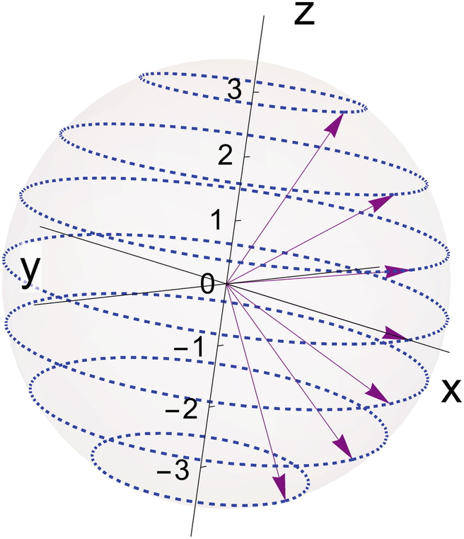
Figure 3:A vector representation of the seven possible vector orientations for an electron with orbital angular momentum quantum number
Example #2
An electron in an atom has orbital angular represented by . There are 5 possible orientations of that vector represented by 2, 1, 0, 1, and 2.
The form of and are the same for other types of angular momentum. All we have to do is replace the quantum numbers representing orbital angular momentum with the quantum numbers that represent the type of angular momentum we are interested in. In the next few sections, we are going to expand our discussion to talk about electron spin, the total electronic angular momentum (orbital + spin), the total orbital angular momentum of multiple electrons in an atom, and more. Each of the above examples of angular momentum will have two quantum numbers associated with it, one for magnitude and one for the z-component (cone height). For example, electron spin will have quantum numbers s and . The formulas for electron spin are and . While the quantum numbers for orbital angular momentum are integers, we will find that the other types of angular momentum quantum numbers can be either integers or half-integers. But they all use the same two formulas and tell us the same information, magnitude and z-component (cone height).
7.5 Adding Angular Momentum Vectors Together
Imagine you had 2 electrons in your atom. Each of those electrons has orbital angular momentum. We want to ask the question, “What is the total orbital angular momentum of the system?” To answer that question, we need to add together two quantum mechanical vectors. As an example, suppose we have an electron with the magnitude of the orbital angular momentum vector represented by (Fig. Figure 2 with 3 possible orientations) and a second electron with (Fig. Figure 3 with 7 possible orientations). We want to add these two vectors together as in Fig. Figure 1, but we have to be thoughtful for two big reasons: (1) the vectors are really more like “vector cones” and (2) there might be incompatible observables we have to think about.
While the math is surprisingly complicated, the result is quite nice:
where L is the quantum number for the composite system. For each value of L, there are possible projections represented by the quantum number . This might be, understandably, confusing. So, let’s unpack this statement using our example of and .
If we add together two quantum mechanical vectors whose magnitudes are represented by quantum numbers and , the total angular momentum of the system will be represented by new quantum numbers L and . The math shows there are multiple possible magnitudes one can get when adding two angular momentum vectors together. However, the new cones for L and follow the same rules that we have been working with: L tells us the magnitude of the angular momentum for the system and tells us the component (or height of the cone). From the math, the largest possible magnitude of L is given by , which is in the thought experiment we are working through. The smallest possible magnitude is , or for the example we are working on. To find all possible values of L, we make a list that starts with the smallest value and continually add 1 until we reach the largest value. In this case L can equal 2, 3, or 4.
To put it another way, there are three different orientations for and seven different orientations for . Depending on the orientations, adding those two angular momentum vectors results in different possible magnitudes. Working through all possible combinations results in three possible magnitudes. For each possible magnitude, there are different orientations (cone heights). In this example, the individual orbital angular momentum vectors can add together to make (5 possible cones with the same length vector ), (7 possible cones with the same length vector ), and (9 possible cones with the same length vector ).
After all the math, there are possible cones. This makes sense since the original vectors had 3 and 7 possible orientations, and . However, I want to caution you in that the new cones are not constructed simply by taking one cone chosen from and one cone from and adding them together. This is because the z-components of the individual electrons are incompatible with the z-component of the composite system. So, the new cones, which we will call the basis set for the composite system, are a superposition of all the cones from the individual electrons, which we call the individual electron basis set. The complicated math, which we skip in this book, tells us the amplitude or amount that we need from each of the individual electron basis set to construct the new composite system basis set. We will explore this more in Sect. 7.5.1 Compatible or Incompatible?.
Another example: Suppose and . The largest value for L is , and the smallest value is . Therefore, L can have values of 2, 3, 4, 5, 6, 7, or 8. For each value of L, there will be different orientations represented by the quantum number . If , there are 7 possible vector cones represented by , 2, 1, 0, 1, 2, and 3.
Quick problem (the answers are in the footnotes[4]):
Suppose and .
(a) How many projections are there for ?
(b) How many projections are there for ?
(c) How many possible cones can we add together from part (a) and part (b)? In other words, what is the size of the individual electron basis set?
(d) What values of L are possible?
(e) For each value of L, how many projections are there?
(f) Add up all the possible projections from part (e).
The answer to (c) should match the answer in (f).
7.5.1 Compatible or Incompatible?
For just these two electrons, we have a bunch of quantum numbers floating around. Each quantum number corresponds to something we can measure. For these two electrons, we have six quantum numbers: , , , , L, and . Which of these represent compatible observables? Is there something we can measure that will disrupt the value of another observable? As learners of quantum mechanics, this is important to keep track of.
All of the magnitudes are compatible with everything. If we know , , and , we can measure any of the observables represented by the six quantum numbers without disrupting future outcomes of magnitude measurements. However, the composite z-component is incompatible with the z-components of the individual electrons, and . Therefore, we can know either the z-component of the system or the z-components of the individual electrons, but not all three at the same time. The z-components of the two individual electrons are compatible with each other. So, if we know the z-component of the system and want to know what we might measure if we were to measure the z-component of the individual electrons, we have to write the state of the composite system as a superposition of states from the individual electron basis states. The concept remains the same; we would just have to do the math to find the amplitudes.
Generalization and Summary
The above discussion is true when adding any two quantum mechanical angular momentum vectors together. Suppose we have two angular momentum vectors and . Their magnitudes are represented by quantum numbers A and B, while their z-components are represented by and . We want to add and together to get . The possible values for the quantum number representing the magnitude of are:
For each value of C, in integer steps. The compatibility of the observables is as follows:
The magnitudes are always compatible with everything.
The z-components of the individual angular momenta are compatible with each other.
The z-component of the summed angular momentum is incompatible with the z-components of the individual angular momenta.
7.6 Other Types of Angular Momentum
An electron, whether it is in an atom or free, always has spin. The quantum numbers for spin are s and for the magnitude and orientation (cone height), respectively. For an electron, always, so the possible orientations are always or . From tradition, we call “spin up” and “spin down”.
If the electron is in an atom, it can also have orbital angular momentum. We can add orbital angular momentum and spin together and ask the question, “What is the total angular momentum of that electron?” This new total angular momentum of the electron is represented by the quantum numbers j and . Using our new rule (Eq. (5)), the possible magnitudes of the total are represented by in integer steps. Thus, if and , j can be or . As before, can be any value between and in integer steps, can be any value between and in integer steps, and can be any value between and in integer steps. Knowing the quantum numbers j, , and s tells us the magnitude of the angular momentum vectors. Knowing , , and tells us the orientation of each of their respective angular momentum vectors. However, is incompatible with and .
Here is a table summarizing all of the current types of angular momenta for a single electron in an atom (QN means quantum number):
| Type | QN | Rule | Formula |
|---|---|---|---|
| Orbital | Zero or positive integer | Magnitude: | |
| to in integer steps | Cone height: | ||
| Spin | s | For a single electron, | Magnitude: |
| and | Cone height: | ||
| Total electronic | j | Zero, positive integer, or half-integer | Magnitude: |
| to in integer steps | Cone height: |
We now have all the building blocks we need to add together as many angular momentum vectors as we need. We first add two together to come up with the new possible quantum numbers and projections for this composite system. Next, we treat the composite system as its own individual angular momentum and add a third angular momentum. Then keep going until you have accounted for all electrons in your atom. The magnitudes of each angular momenta will be compatible with everything. The z-component of any summed angular momentum will be incompatible with the two individual angular momenta.
In practice, we don’t go through all this effort. As we will see in Chap. 8. Electronic Structure and Atomic Notation, there are shortcuts we can take and databases that tell us all we need to know. For atoms with more than 1 electron, we do not keep track of subscripts (i.e., electron 1, electron 2, etc.), we simply ask the question “how much orbital, spin, and total electronic angular momentum do all of the electrons have?” The formulas and ideas are identical, but we use capital letters when we ask how much angular momentum the electrons as a whole have:
| Type | QN | Rule | Formula |
|---|---|---|---|
| Orbital | L | Zero or positive integer | Magnitude: |
| to in integer steps | Cone height: | ||
| Spin | S | Zero, positive integer, or half-integer | Magnitude: |
| to in integer steps | Cone height: | ||
| Total electronic | J | Zero, positive integer, or half-integer | Magnitude: |
| to in integer steps | Cone height: |
All of the magnitudes are compatible with everything. However, is incompatible with and .
Something Super Annoying, But Unfortunately Super Important
Historically, we assign letters to orbital angular momentum quantum numbers. A system with no orbital angular momentum has the quantum number (or for a single electron) is given the letter designation S (or s for a single electron). But, S and s are also the quantum numbers for spin. They are both angular momenta, but very different types. Technically the quantum numbers are italicized and the letter designations are not, but that is not a rule everyone follows. Below is a table with quantum numbers, the letter designation, and double uses with other types of angular momentum:
| Orbital quantum number | Letter designation | Other uses |
|---|---|---|
| S (s) | S and s are also used for spin | |
| P (p) | ||
| D (d) | ||
| F (f) | F is also used for nuclear angular momentum | |
| G (g) |
I admit it is extremely annoying to have orbital angular momentum represented by letters that also mean different types of angular momentum, but it is unfortunately the way of spectroscopy. It takes some getting used to.
The Nucleus
The nucleus can also have angular momentum. Traditionally, this is called nuclear spin, but that is a bit of a misnomer. The angular momentum of the nucleus comes from the spin of the protons and neutrons as well as any orbital angular momentum of those nucleons. So, nuclear spin should really be called total nuclear angular momentum but no one uses that phrase. Nuclear spin has the quantum numbers I and . Nuclear spin can be added to the total electronic angular momentum find the total angular momentum of the atom. The total angular momentum is represented by the quantum numbers F and , where F is found from J and I using Eq. (5):
As always, is incompatible with and .
So, if an atom has nuclear spin, our table gets a bit longer:
| Type | QN | Rule | Formula |
|---|---|---|---|
| Orbital | L | Zero or positive integer | Magnitude: |
| to in integer steps | Cone height: | ||
| Spin | S | Zero, positive integer or half-integer | Magnitude: |
| to in integer steps | Cone height: | ||
| Total electronic | J | Zero, positive integer, or half-integer | Magnitude: |
| to in integer steps | Cone height: | ||
| Nuclear spin | I | Zero, positive integer, or half-integer | Magnitude: |
| to in integer steps | Cone height: | ||
| Total Atomic | F | Zero, positive integer, or half-integer | Magnitude: |
| to in integer steps | Cone height: |
We will explore nuclear spin more in Chap. 9. Hyperfine Structure.
The Photon
The photon has intrinsic angular momentum as well. Photon spin is the quantum mechanical description of light polarization, and it has a quantum number of 1. In Chap. 1. Introduction to Atoms and Light, we talked about how light can be linearly polarized, circularly polarized, or elliptically polarized. That statement is for a laser beam, which is composed of many photons. A single photon is circularly polarized. To help visualize this, imagine a photon traveling straight towards you. The photon would be rotating either clockwise or counterclockwise. To be clear, a photon is not actually rotating just like the electron is not actually spinning like a top. However, both the electron and the photon behave and interact with other particles as if they are spinning or rotating. If it is spinning counterclockwise, the height of the cone is (the z-component to photon spin with a quantum number of +1). If the photon is spinning clockwise, the height of the cone is .[5]
Circularly polarized light just means that all the photons are rotating in the same direction. A laser beam composed of photons coming towards you that are all rotating clockwise is said to have left (or left-handed) circularly polarized light. A laser beam composed of photons that are all rotating counterclockwise is said to have right (or right-handed) circularly polarized light. To get linearly polarized light, you need to have equal amounts of photons spinning clockwise and counterclockwise. Elliptically polarized light has an imbalance between the number of clockwise and counterclockwise photons.
7.7 A Bit More on Compatible and Incompatible Observables
Every quantum number in every table in Sect. 7.6 Other Types of Angular Momentum is something we can measure. Consider the hydrogen atom, which has a single electron. For now, we will ignore the fact that the nucleus of a hydrogen atom has angular momentum (this is the topic of Chap. 9. Hyperfine Structure so we will revisit compatible and incompatible observables again in that chapter). Here is a list of things we can measure: , , s, , j, and .
Technically, we could also measure L, , S, , J, and , but, since the hydrogen atom has only a single electron, measuring, for example, the total orbital angular momentum of all the electrons is the same as measuring the orbital angular momentum of the single electron in the system.
We want to ask the question, which of these observables is compatible with energy? In other words, if the hydrogen atom was in an energy state, what other properties could we measure and still leave the electron in that same energy state? The answer is:
Compatible with energy: , s, j, and
Incompatible with energy: and
That means if the system was in an energy state and we measured the z-component of the electron’s orbital angular momentum, the system is now in a superposition of energy states. But what makes and incompatible with and energy? While it isn’t obvious why and are incompatible with the energy state, we can visualize why they are incompatible with . Fig. Figure 4 visualizes the incompatibility. This figure shows the addition of two angular momentum cones. Since is compatible with the energy state, we will define the z-axis to be along the cone for j. I want to point out a few things. First, notice that the cones for both and s are tilted with respect to the z-axis. This means that the height of those two cones (i.e., the result of a measurement of or ) are no longer perfect projections onto the z-axis. In other words, if we measured the z-component of spin with respect to this z-axis, we will be in a superposition of the basis set. Compare this to the measurement of the z-component of j. The cone for j has a rim that is constant along the z-axis, so we will always measure the same value of . Since is compatible with the energy state, measuring or would also put the system into a superposition of energy states.
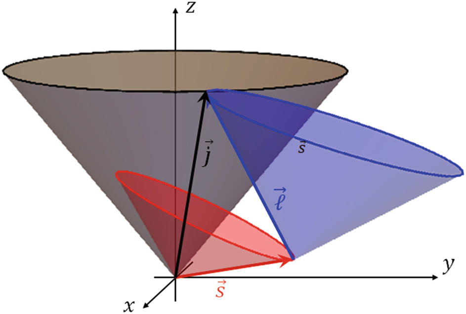
Figure 4:An example of adding together a spin cone and a orbital angular momentum cone to get the total electronic angular momentum cone. Notice that the z-component of both the spin and orbital angular momentum cones is not the same value at all points of the cone tops. This means the z-component does not have a specific, discrete value, which means that both the z-component of spin and the z-component of orbital angular momentum are incompatible with the z-component of j
The second thing I would like to point out is that the length of the both s and are constants. If we were to measure the slant height of either cone, we will always get the same answer. In other words, both s and are compatible with j and energy.
To clarify which observables are compatible with the energy states, I’ll reintroduce the quantum number for energy, n, from Chap. 6. Quantum Mechanics vs. Classical Physics. We use the quantum numbers representing those observables that are compatible with energy in a ket: . We will discuss these quantum numbers and their relationships to electron shells in more detail in Chap. 8. Electronic Structure and Atomic Notation. If the electron in the hydrogen atom is in an energy state represented by one of these kets, we can measure any of those observables and still be in that same energy state. If we measured or , the system would be in a superposition of energy states.
Let’s solidify this idea with a couple of examples. We will do Example #1 together, and then you should do Example #2.
Example #1
How many states will there be for the electron in a hydrogen atom that has , , and ?
To start this problem, let’s first calculate what values of j are possible. j can range from to in integer steps, so j can be or . If , then can be or . If , then can be 3/2, 1/2, -1/2, or -3/2. Therefore, there are 6 energy states with , , and . Using the notation , these states are: , , , , , and .
The above math tells us that there is an energy state in the hydrogen atom that is represented by, for example, the quantum numbers . If the hydrogen atom is in this state, it has a defined magnitude of orbital angular momentum (in this case ), a defined magnitude for spin, a defined magnitude for the total electronic angular momentum, and a defined z-component for the total electronic angular momentum. That state does not have a well defined z-component of orbital angular momentum nor a well defined z-component of spin. We can measure any observable compatible with energy and the system will stay in the state. However, if we measure or , the system will be in a superposition of energy states.
Example #2
The electron in the hydrogen is in the state .
(a) What will we measure for the electron’s orbital angular momentum, the electron’s spin, the electron’s total angular momentum, and the electron’s z-component of the electron’s total angular momentum?
(b) If we measured the z-component of the electron’s orbital angular momentum, what might we get?
The solutions are below the crossword.
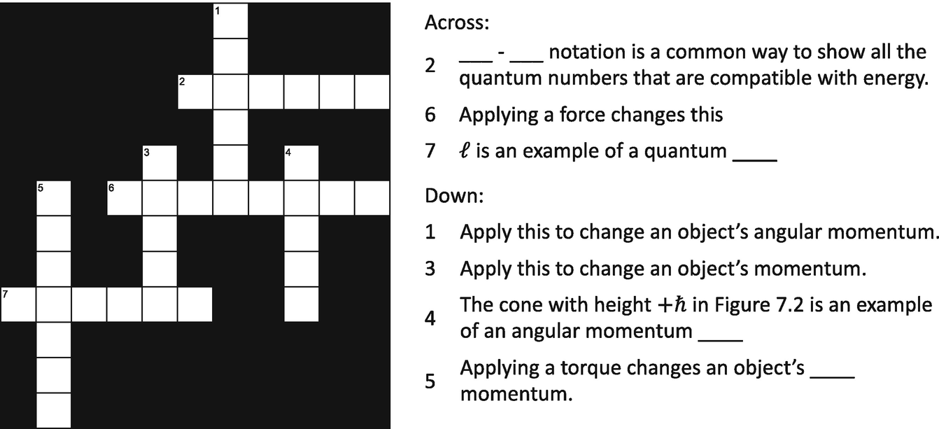
Solution
(a)
We will measure with 100% probability
We will measure with 100% probability
We will measure with 100% probability
We will measure with 100% probability
(b) We would measure either , 0, or with different probabilities. We would need advanced math to calculate those probabilities, so I will just emphasize that we will not measure a definite value for the z-component of the electron’s orbital angular momentum. After the measurement, the system will no longer be in the state , but a superposition of energy states. If we now went back and measured j, we might get or with hard to calculate probabilities.
7.8 Problems
Remember that in quantum mechanics, an electron is not like the moon orbiting the earth but more like a wave that is surrounding the nucleus. We are just using the moon and earth as an analogy to introduce angular momentum.
There are, at least, two things in physics that really boggle my mind. The first is spin. The second is something called the fine structure constant, which you should Google if you want your mind blown!
I, personally, like using cones. But, as long as you understand the concepts, it doesn’t matter which version you use.
(a) 3; (b) 5; (c) ; (d) 1, 2, or 3; (e) 3, 5, or 7; (f) 15.
Because the photon has no mass, the math, interestingly, forbids a z-component of 0.