Abstract
In this chapter, we explore the differences between quantum mechanics and classical physics, focusing on three main ideas: compatible and incompatible observables, states of an observable, and the superposition of states. By examining these concepts, you will gain insight into how measurements impact quantum mechanical systems and the ideas behind the uncertainty principle.
Keywords: Quantum states, Observables, Compatible observables, Incompatible observables, Uncertainty principle, Superposition, Harmonic oscillator, Basis sets completeness, Energy basis
Learning Goals
By the end of this chapter, you should be able to understand:
the importance of discrete energy states in quantum mechanics.
compatible and incompatible observables.
basis sets.
superposition of states.
I’m often asked some variation of the question, “What is the difference between quantum mechanics and classical physics?” This is a great question! After teaching quantum mechanics many times and having numerous conversations with other atomic and nuclear physicists, I believe the best way to introduce the difference to new learners is to first understand two concepts: states and superposition. By grasping these two ideas, we can begin to explore why quantum mechanics is essential for explaining the world of the super small.
A note from Will: Many concepts discussed in this chapter are based on the orthodox or Copenhagen interpretation of Quantum Mechanics. Although it is the most popular interpretation, other interpretations exist, such as the many-worlds interpretation, de Broglie-Bohm pilot wave theory, and various collapse theories including Ghirardi-Rimini-Weber (GRW) theory and Continuous Spontaneous Localization (CSL). This remains an active area of exploration for many physicists and philosophers.
In addition, there are a few places where I simplify things a bit to make sure we focus on the main concepts. Finding the balance between 100% correct and still keeping things accessible was a challenge. For example, there are places where I will write a sum of functions where it should technically be an integral, but since calculus is not required for this book, I purposefully chose to leave them as sums to help us explore the concepts. For equations that should be integrals, I include a footnote to indicate that. For those who have not taken calculus, the ideas we discuss are still correct! We are just going to simplify the math a bit.
The other concept I simplify a bit is concerning compatible observables and sharing states. However, after discussions with my physics pedagogy friends, I decided to keep that language instead of exploring the delicate topic of projections and subspaces. For the advanced readers, keep this in mind. For new learners to quantum mechanics, this chapter is for you! If in the future you decide to learn more advanced quantum mechanics (and I hope you do!), please come back to this chapter to explore the subtleties of “commutation” and “subspaces.”
6.1 What Is a State?
Definitions
Momentum: A property of an object that is moving. For a classical object like a baseball, the formula for momentum is , where p is the object’s momentum, m is the object’s mass, and v is the object’s velocity. An object’s momentum will change if something acts on the object from the outside. The larger an object’s momentum, the harder it is to stop. The unit of momentum is .
Observable: Something we can measure experimentally. Observables include, but are not limited to, energy, position, momentum, and angular momentum (angular momentum is the topic of Chaps. 7. Angular Momentum and 8. Electronic Structure and Atomic Notation).
Physical systems, such as atoms, can exist in various conditions. They can be excited or relaxed, located in different places, moving or at rest, and so on. We describe these different conditions as “states,” and use a mathematical “state function” to specify the exact state of a system at a given time.
As we talked about and explored in Part 1 of this book, atoms have discrete energy states.
Two minute question: What does that mean?
Here is my answer: If we measure the energy of a quantum mechanical system, we will always find the system to have one value from a set of specific energies. The whole purpose of Part 1 of this book was how we experimentally find the energy between two of these discrete energy states. An electron in an atom can have energy , , , etc. We will never find the electron with any other energy. We represent these discrete energy states in energy level diagrams throughout Part 1 of this book. Figure Figure 1 is a copy of Fig. Figure 12 as a helpful reminder. This is so important that I want to say it again: An electron in an atom can have energy , , , etc. We will never measure the energy to be somewhere between and .
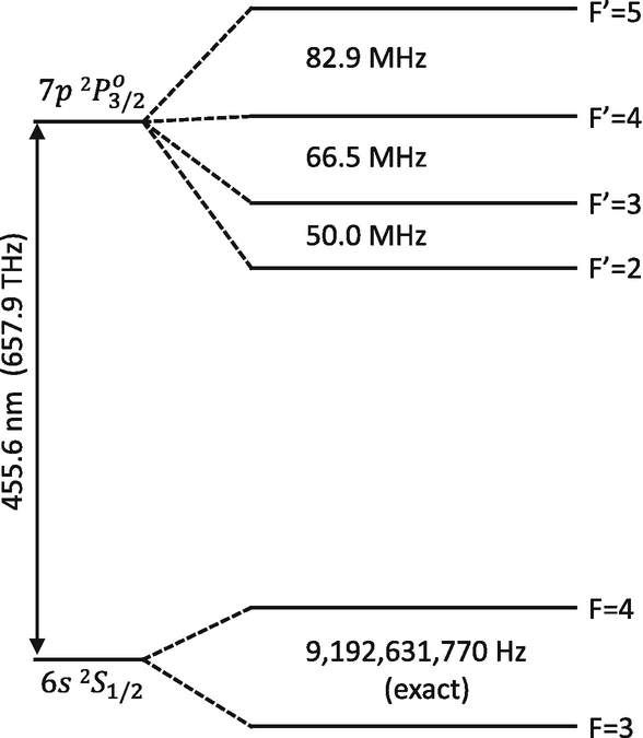
Figure 1:A simplified energy level diagram for the transitions in cesium-133 near 455.6 nm
Everything we can measure, which we call an observable, is represented by a state. The state of an observable is described by a mathematical function. Examples of things we can measure include energy, position, and momentum. As such, there are energy states, position states, and momentum states. Every energy we can measure is associated with some energy state. For example, suppose a system is in an energy state described by the state function . If we measure the energy of that system, we will find the system has energy . We will never measure any other value for energy. Often those states are discrete (like the energy of an electron in an atom) and sometimes they are continuous (like the position of an electron hanging out by itself in free space). If we measure an observable, the quantum mechanical system will be in a state corresponding to that observable after the measurement.
To help explore the idea of energy states, we will use a classical analogy that will serve as a helpful visualization tool. Imagine a string fixed at both ends, vibrating to create different standing waves, see Fig. Figure 2. These are the same standing waves we discussed in Chap. 1. Introduction to Atoms and Light as a means of illustrating wave interference.
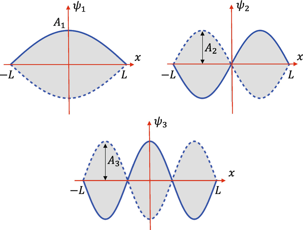
Figure 2:The first three standing waves of a one dimensional rope or slinky. For this example, the rope is fixed at and
Now, let’s shift our perspective from the classical realm to the quantum mechanical domain. If we were to treat this system quantum mechanically and measure its energy, we’d find discrete energy levels. These energy levels correspond to specific configurations of the standing wave—for instance, one loop, two loops, three loops, and so on as shown in Fig. Figure 2. Unlike in the classical scenario where the wave can have any arbitrary energy, in the quantum realm, the energy is constrained to certain discrete values.
To formalize this, we use mathematical expressions known as wavefunctions,[1] denoted by the lowercase Greek letter psi (). Each wavefunction, labeled as , corresponds to a particular energy level, which will have energy . The wavefunction encapsulates the behavior and properties of the system at that energy level. In quantum mechanics, the equation we use to calculate the wavefunctions and energies is called the Schrödinger equation. The Schrödinger equation is a partial differential equation and solving it for a system provides not just the spatial form of the wavefunction, but also how they evolve in time. If you take a quantum mechanics class, you will spend a good amount of time solving the Schrödinger equation for different physical scenarios.
Returning to our example of the vibrating quantum mechanical string, we can now describe the wavefunctions for specific energy states. The wavefunction corresponds to the state with one loop of energy, denoted by . Its functional form, see Fig. Figure 2, is described by , where represents the amplitude and 2L denotes the length of the string. Similarly, represents the state with two loops and has a functional form of .
Summary So Far
If a quantum mechanical system has a particular energy, we say the system is in an energy state. Mathematically, that energy state is described by the wavefunction . If a quantum mechanical system is in an energy state described by the wavefunction and we measure its energy, we will measure the system’s energy to be . We will never measure anything else.
For the example in this section, n represents how many loops of energy the system has, so is the third picture in Fig. Figure 2. In bra-ket notation, see Sect. 3.6 Example, we would write either or . There are other quantities (obersvables) that we can measure, and each thing we measure can change the shape of the wavefunction. Figure Figure 3 shows an example of three position states. If we measure the position of a quantum mechanical particle, we would find the particle somewhere between the start and end of the string. Mathematically, we label those position states with a subscript, like . Notice that the position wavefunction is zero everywhere except for where the particle was measured. For the first example, the particle was measured to have a position at . For the second example, the particle was measured to have a position at .
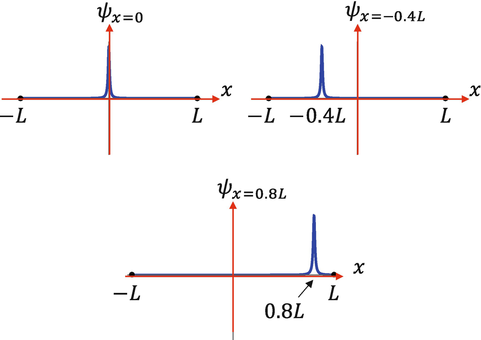
Figure 3:Examples of 3 different position states. Each position state has a specific position associated with it
Super Important
For this quantum mechanical system, the energy states are not position states. They look completely different.
If we measure the energy of a quantum mechanical system, the system will be in an energy state, for example one of the energy states shown in Fig. Figure 2. If we measure the position of a quantum mechanical system, the system will be in a position state, for example one of the position states shown in Fig. Figure 3. These are not the same states!!
That last sentence is super important. If I told you a quantum mechanical system had energy , that statement comes with the understanding that our system is in an energy state ( or ) that has energy .[2] If the system was in the energy state and I were to ask, “Where exactly is the quantum mechanical particle?”, we wouldn’t be able to answer that question. The wavefunction, see the graph with 3 loops in Fig. Figure 2, is spread out over the entire range from to and this is not a position state, see Fig. Figure 3. While we can’t state precisely where the particle is, we can, as we will see in Sect. 6.3 Superposition of States, answer the question, “What are the probabilities of finding the particle in various locations?”
Likewise, if I told you a quantum mechanical particle was at a position , that statement comes with the understanding that our system is in a position state with a location at . If I were to ask, “What is the energy of the quantum mechanical particle?”, we wouldn’t be able to answer that question exactly because the system is not in an energy state. Like with the example given above where we know the energy but not the exact position, we will be able to answer the question, “If the particle is in the position state , what are the probabilities of finding the particle with a particular energy?”
Stepping Back
Take a look at one of the energy states shown in Fig. Figure 2 and ask the question, “Where is the particle?” The best you can answer is, “The wavefunction is spread out from to . It is not at any single location.” The energy has a single value, but the exact position is unknown.
Far less intuitive is if we repeated this thought experiment with position states. Take a look at one of the position states shown in Fig. Figure 3 and ask the question, “What is the energy of the particle?” Our intuition tells us there is an answer to this question. However, in quantum mechanics, a particle only has a specific energy if it is in an energy state. A position state is not an energy state. The best you can answer is, “The energy is spread out. It does not have a single value.”
Take as much time as you need to try and understand that last paragraph. That last paragraph is very counterintuitive to our everyday experience. In classical physics, if a car is traveling down the road, I can tell you its position and energy. In quantum mechanics, we cannot know both. If the energy is well defined, it is in an energy state. If the position is well defined, it is in a position state.
There are two really important things to take away from this section:
If we measure the energy of a quantum mechanical system, that system will be in an energy state with a specific energy. If we measure the position of a quantum mechanical system, that system will be in a position state with a specific position.
Energy states and position states are not the same. They look completely different. If we measure the energy of a system, the system will now be in an energy state and the position of the particle is spread out. Similarly, if we measure the position of a system, the system will now be in an position state and the energy of the particle is spread out.
6.2 Compatible vs. Incompatible Observables and the Uncertainty Principle
Definitions
Incompatible observables: If two observables cannot be precisely measured at the same time, they are called incompatible. Measuring one observable changes the system, making subsequent measurements of the other observable unpredictable.
Compatible observables: If two observables can be precisely measured at the same time, they are called compatible. Measuring one observable does not change the system in a way that affects the measurement of the other observable. Remeasuring either observable will return the same value as initially measured.
We have learned that for quantum mechanical systems, energy and position are incompatible observables. If the system is in a position state, it is not in an energy state and vice versa. If we measure the position of the system, it is now in a position state. Since that is not an energy state, we cannot predict the exact outcome when we measure the system’s energy.
If there are two observables that share the same set of states, we say that they are compatible observables. For the system in Sect. 6.1 What Is a State?, there are, unfortunately, no compatible observables, but we will be able to explore compatible observables using systems in Chap. 7. Angular Momentum. So, for now, let’s just suppose there is some other observable that is compatible with energy. Let’s call that observable A, described by the wavefunction with possible measured values . If we measure the energy of a quantum mechanical system, the quantum mechanical system will now be in an energy state. Let’s say we measured the energy of the system to be , which is the third picture with three loops in Fig. Figure 2. Now we measure A and obtain . If we went back and measured energy, we will find that the system is still in the state with three loops with energy . Next, we measure A. If energy and observable A are compatible, we will measure . This is because two compatible observables share a set of states. In other words, if the energy state has the wavefunction with three loops (), and we measure A, we will find and that the wavefunction is unchanged. It still has three loops.
The Uncertainty Principle Part 1
The compatibility or incompatibility of two observables is summarized by the uncertainty principle. If two observables are compatible, they share a set of states. We can measure both observables repeatedly and obtain consistent values. If the two observables are incompatible, they do not share a set of states. Measuring one observable disrupts the outcome of the measurement of the other.
As you see, states are extremely important in quantum mechanics. Every observable has a set of associated states. Each energy state corresponds to a specific energy. If we measure the system’s energy, it will be in one of those states with the associated energy. Similarly, measuring position, momentum, or any other observable places the system in one of the states for that observable. Some observables share a set of states (they are compatible, and subsequent measurements do not alter the previous values), while others have different states (they are incompatible, and knowing one means we don’t know the other).
6.3 Superposition of States
Definitions
Superposition: A concept in math and physics that says a function can be constructed as the sum of two or more other functions.
Basis set: All of the states for a particular observable for a particular system. All of the possible energy states (for example, 1 loop, 2 loops, 3 loops, 4 loops, etc. for the vibrating quantum mechanical string shown in Fig. Figure 2) make up the energy basis set for that system. Similarly, all possible position states (Fig. Figure 3 shows a few position states for the vibrating quantum mechanical string) make up the position basis set.
Another really important concept to understand is superposition. Let’s explore superposition through an example. Suppose we measure the position of a quantum mechanical system and find it in the position state shown in the top right picture of Fig. Figure 3. Although this is not an energy state, we can still infer some information about the system’s energy. The concept of superposition will allow us to determine the probability that, upon measuring energy, the system will have one loop, two loops, three loops, etc.
What we will do is “build” a position state by cleverly adding together all of the energy states. Using more mathematical language, we will construct a position state from a superposition of states from the energy basis set. Although this sounds strange–since energy states have loops and the position state we are interested in is a spike–we can, remarkably, build a spike from loops!
To help understand this concept, let’s do a thought experiment where we put the system into a state that isn’t a position state, but is mathematically simpler, in order to explore the concept of superposition. At the end of this section, I will show graphs to build the position state seen in the top right of Fig. Figure 3 from the energy basis set. The example state we will use to explore superposition is shown in Fig. Figure 4a.
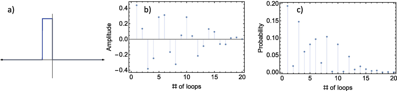
Figure 4:(a) The state for our thought experiment. (b) The amplitude of each energy state needed to construct the state. (c) The probability that, upon measurement of energy, we find the system in a particular energy state
Mathematically, the energy states (those shown in Fig. Figure 2 plus all the other possible energy states) can be added together to construct the desired state. More formally, we say that a state can be constructed as a superposition of the energy basis set:
where is the amplitude of that is mathematically determined to reconstruct the desired state . The set of all states is called the energy basis set. This equation represents the concept of superposition. We are constructing a specific state from a superposition of states from the energy basis set. The math required to calculate the amplitudes is complicated and requires integrals, so I am just going to show you the results of the math in Fig. Figure 4b. In practical terms, we start with the energy state with 1 loop (left picture in Fig. Figure 2) and set the amplitude to 0.44. Next, we take the energy state with 2 loops (middle picture in Fig. Figure 2), set the amplitude to 0.14, and add it to the energy state with 1 loop that had an amplitude of 0.44. We then take the energy state with 3 loops, set the amplitude to -0.38, and add it to the first two energy states. This process repeats, and the more energy states we include, the closer we get to the actual state. This is illustrated in Fig. Figure 5. Adding the first two energy states together (top row) with the appropriate amplitude doesn’t resemble the desired state, but after adding the first 30 energy states (third row), the resultant graph starts to look like the desired state. A superposition of the first 200 energy states (bottom row) results in a close reconstruction. Remarkably, loops can construct this state! Even more astonishingly, you can create any state you want (as long as it is a well-defined single-valued function) from the energy basis set. In other words, you can construct any state from a superposition of energy states.
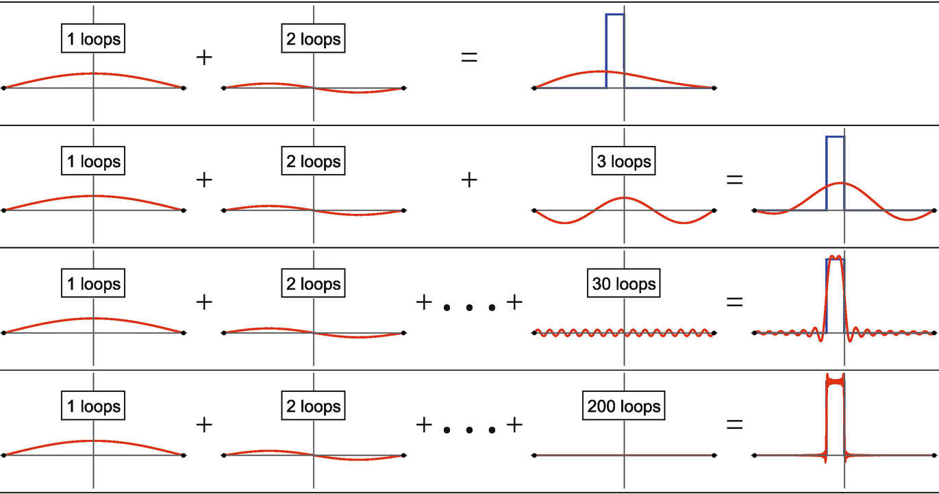
Figure 5:An illustrative example of adding more and more energy states together to build the desired state. The amplitude of the energy state with 1 loop is 0.44, the amplitude of the energy state with 2 loops is 0.14, 3 loops has an amplitude of -0.38, etc. For the bottom row, the energy state with 200 loops looks flat to our eye, but it has a very small amplitude of 0.019
Since we can construct a state out of energy states, we say that the state is a superposition of states from the energy basis set. Similarly, we could construct an energy state from a superposition of states from the position basis set. All we need is some mathematical method to determine the amplitudes of each of the position states so that when we add them all together we get the desired energy state.
In quantum mechanics, this is a very general idea. We can always construct a single state from any basis set using a superposition of states from another basis set. For example, we can construct a momentum state from a superposition of states from the position basis set, a position state from a superposition of states from the momentum basis set, a momentum state from a superposition of states from the energy basis set, and so on. This is a neat math trick, but is it useful? It is perhaps the most useful math trick in all of quantum mechanics.
Suppose we are in the state given by Fig. Figure 4a. Now we want to measure the energy of the system. The amplitudes given in Fig. Figure 4b can be used to calculate the probability that, upon measurement of energy, we will find the system in a particular energy state. All we need to do is square that amplitude. For example, the amplitude of the first energy state (1 loop) is 0.44. The probability that, upon measurement of energy, we find the system with one loop of energy is , or 19%. The amplitude of the third energy state (3 loops) is -0.38. The probability that, upon measurement of energy, we find the system with 3 loops of energy is , or 15%. The probabilities are given in Fig. Figure 4c. This rule is universal. If the system is in a particular energy state and we want to measure position, there is an associated probability for where we would find that quantum mechanical particle. Those probabilities are found by first writing the energy state as a superposition of all the position states from the position basis set with the correct amplitudes. Squaring those amplitudes[3] will tell you the probability that, upon measurement of position, a quantum mechanical particle will be found at a particular position.[4]
The above discussion is for two incompatible observables. The two incompatible observables have distinct basis sets, one for each observable. Measuring one of the observables puts the system in a single state from that observable’s basis set. However, that single state can be constructed from a superposition of states from the other basis set. But, what if we had two compatible observables? Let’s recap some of the important concepts:
If the two observables are compatible, they share a basis set.
If we measure one observable, the system is now in a state of that observable.
If the two observables are compatible, measuring one observable does not change the system in a way that affects the measurement of the other observable.
Interestingly, we can use superposition to answer this question. Suppose energy and our made up observable A are compatible observables. We measure the energy of the system and find the system has energy . The system is now in the energy state , which is also the same as . Let’s write that energy state as a superposition of states from the basis set for observable A:
For the system we are exploring, building the energy state from a superposition of A states is really easy! and are literally the same sate. The probability that, upon measurement of A, we find the system with (the value associated with ) is 0%. The probability that, upon measurement of A, we find the system with value (the value associated with ) is 100%. The system is already in that state! Constructing the energy state from the A basis set is easy because there is one state from the A basis set that perfectly matches the energy state.
Now that we have explored the concept of superposition, let’s build a more realistic position state, similar to the top right graph in Fig. Figure 3, from the energy states. Figure Figure 6 shows the mathematical results needed to construct that position state from the energy basis set. As you can see, we needed at least twice as many energy states to get a good approximation for a position state. Despite needing many more energy states to accurately reconstruct a single position state, the result remains the same: if the quantum mechanical system were in that position state and we measured its energy, we could get many different answers with probabilities given by the squared amplitudes.
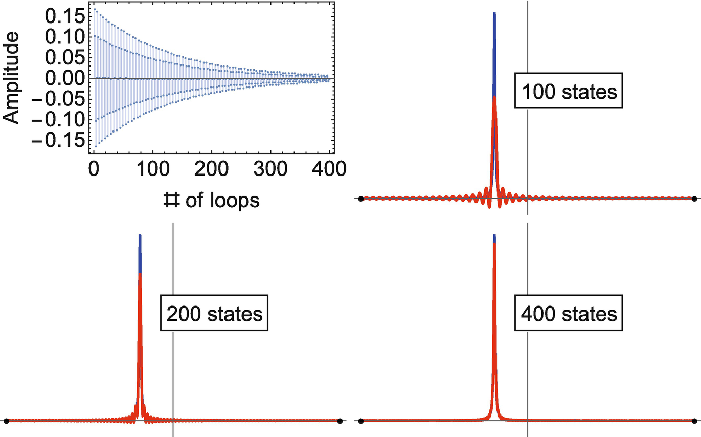
Figure 6:Constructing the position state from the middle picture in Figure Figure 3. We need over 400 energy states to build this one state! Notice the position state in blue is noticeably taller than the reconstructed states even when we use the first 200 energy states. The position state is still a bit taller even with 400 energy states!
The Uncertainty Principle Part 2
Measuring an observable puts the system into a single state for that observable and in a superposition of states for a second observable. If a second observable shares states with the basis set of the first observable, the value of that second observable is already determined. We can measure both quantities as many times as we’d like, and we will never change the state of the system. We will always get the same answer as the first time we measured.
If the two observables have different basis sets, knowing the value of one observable does not inform you of the value of the other. These observables are incompatible. Measuring one observable places the system in a superposition of states for the other observable where none of the amplitudes are 1. Therefore, the state of the second observable after measurement is probabilistic.
States and superposition of states are core concepts in quantum mechanics. Let’s summarize the entire chapter using two generalized observables and .
Both and have states associated with them, denoted as and .
The set of states that are needed to describe all possible values for is called the basis set of . The set of states that are needed to describe all possible values for is called the basis set of .
Each state has a measurable value associated with it. If the system is in state and we measure , we will get the value associated with that state, . We will never measure, for example, .
If and are incompatible, they have different basis sets. If they are compatible, they share a basis set.
A state for can be written as a superposition of states for , and vise-versa. For example,
or
The square of the amplitudes in the above equations tell us the probability, upon measurement, we will find the system in that state with the value associated with that state. For example, if the system was in state with value and we measured , the probability the system is now in a particular state of , say state with value , is the amplitude squared, .
Suppose we measured and got . Next, let’s say we measure and get . If and are incompatible and we then re-measure , it is highly likely we will get something other than .
6.4 The Energy Basis Set for a Quantum Harmonic Oscillator
The quantum harmonic oscillator is one of the first quantum systems learners encounter in a quantum mechanics class, and it is a very practical system to study. It can be used to model many physical systems including molecular vibrations, see Fig. Figure 7. Consider two atoms connected by chemical bonds to form a single molecule. A classical model for this system is to have the two atoms connected by a spring. If the two atoms are not moving and the spring is not stretched or compressed, the system would just sit there at rest and not vibrate. However, if the spring is stretched slightly, it tries to pull the atoms back closer together. As the atoms move closer, the spring passes its equilibrium length and compresses. Once compressed, the spring tries to push the atoms apart until it stretches past equilibrium again, and the process repeats. This is an oscillation. In a quantum mechanical version, this system will have discrete energy levels, meaning it will have specific energy states. If the spring from this classical analogy were behaving quantum mechanically, the spring would only oscillate at specific frequencies.
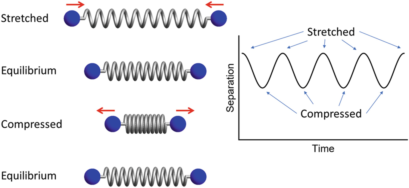
Figure 7:Left: Two atoms connected by a spring. This is a model for two atoms connected by molecular bonds. Right: The separation of the atoms as a function of time
We can use the Schrödinger equation to find the energy states and their energies for the quantum harmonic oscillator. The energy states with the four smallest energies for the quantum harmonic oscillator are shown in Fig. Figure 8. Notice the similarities with the standing waves on a string example in Sect. 6.1 What Is a State?. Although the shape of the states look different, the lowest energy state has 1 loop, the second lowest energy state has 2 loops, etc. If we measure the vibrational energy of a molecule modeled by the quantum harmonic oscillator, we would find the system in one of the energy states such as those shown in Fig. Figure 8. Each state has a defined, discrete energy. All of the same bullet points that summarized Sect. 6.3 Superposition of States are still true! Observables that are compatible with energy, for example the frequency of vibration, have the same basis set, allowing us to measure all compatible observables repeatedly without disturbing the outcome of measuring other compatible observables. Observables that are incompatible with energy have different basis sets. If we measure energy, the system will be in a state from the energy basis set and a superposition of states for the incompatible observable’s basis set. The amplitudes in the superposition formula allow us to calculate the probability of what we will measure for the incompatible observable.
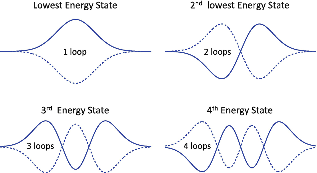
Figure 8:The energy states with the four smallest energies for the quantum harmonic oscillator. Each of these energy states also corresponds to a specific energy or frequency of vibration of the atoms in the molecule
6.5 The Uncertainty Principle Part 3
Reminder Definition
Reduced Planck’s constant (h-bar): ;
The most common explanation of the Uncertainty Principle is about intrinsic limitations to the precision with which pairs of certain physical properties of a particle can be simultaneously known. Let’s connect that idea with what we talked about in this chapter. Suppose a quantum system is in the rectangular state shown in Fig. Figure 4a. This is neither an energy state, a position state, nor a momentum state. However, we now know that we can write this state as a superposition of states from any observable’s basis set.
For momentum, we would write[5]
where are the states making up the momentum basis set. Similarly, we could write the state as a superposition of states from the position basis set:
where are the states making up the position basis set. If the system was in the state shown in Fig. Figure 4a, and we measured momentum, we would get a range of possible values. More specifically, we have a chance of measuring , a chance of measuring , and so on. Equivalently, we would have some average value of momentum. For example, if we had a chance of measuring , the range (or spread) of possible measurements for momentum is 0 while the average value would be . Let’s call the range and the average value we measure . Similarly, if we instead had measured position, we would get a range of possible position measurements, which we will call , and an average position measurement, which we will call .
If two observables A and B are compatible, there is a scenario where . That scenario would be when the system is in a state of A, which also happens to be a state of B since they are compatible. In that scenario, there is no range of measurements for either A or B: and . However, if the system was not in a state of A and B, there would be a range of possible measurements for both observables. Therefore,
This equation covers all possible scenarios for two compatible observables.
Now let’s explore incompatible observables, for example momentum and position. Since momentum and position are incompatible, then there is no situation where . If we did the math to determine the relationship, we would find that there is a minimum possible value to this product. For these two observables, the minimum possible value is
No matter what state you consider, there will always be a range of possible measurements for at least one of the observables. You might be asking yourself the question, “But wait, if the system was in a position state, wouldn’t and thus ?” If the system was in a position state, the range of possible measurements for momentum would be . So, we would have , which is undefined. However, if we were to carefully take the limit as and , the product is still greater than .
For every pair of incompatible observables, the product of the ranges is greater than some minimum value. The result is easier to read for some pairs of incompatible observables than others. For example, Eq. (8) is fairly straightforward: the range of possible measurements of position multiplied by the range of possible measurements of momentum is always greater than or equal to the constant . Other times, the uncertainty principle is harder to interpret. The uncertainty principle for position and energy is
This equation is a bit harder to read. I would interpret it as follows: for a given state, the product of the spread of possible position measurements and the spread of possible energy measurements will always be greater than a constant times the magnitude of the average value of possible momentum measurements. This is a formula that you must be careful with. There are scenarios where , but that does not mean that there is a scenario where position and energy are compatible. This just says that the product of their ranges must be greater than or equal to 0.
6.6 Looking Forward
This chapter solidifies some concepts we explored in the first part of this book while adding some more. Some observables are compatible (i.e., they share a basis set and subsequent measurements do not disrupt the values of the observables) and some observables are incompatible (i.e., they do not share a basis set and measuring one observable puts the system in a superposition of states for the other observable). The next questions to think about are
What observables are compatible with energy?
What observables are incompatible with energy?
We will explore these questions in the next few chapters.
A reflection from Will: This was a really hard chapter for me to write![6] There are so many fun things to explore in quantum mechanics that I had a difficult time narrowing it down to just a few important concepts. So, please take this chapter as an initial introduction. If you choose to go on and learn more about quantum mechanics (and I hope you do!), you can use this chapter as a base to build more understanding. There are many fascinating things to explore like quantum entanglement, Bell’s Inequality, Ehrenfest’s theorem, and the no-cloning theorem, just to name a few. The uncertainty principle also has much more to explore and learn. As with all things worth learning in life,
Problems
In quantum mechanics, we prefer the phrase wavefunction over state function.
As we work through the next few chapters, we will add more parameters to describe the state. Eventually, the state will look something like . The 3 in this example is the n.
For completeness, the amplitudes could be complex numbers, which is something beyond the scope of this book. In the future, if you see an amplitude that is complex, you calculate the modulus squared of the amplitude.
For completeness (again ☺), position and momentum are, mathematically, a bit harder to deal with since their measured values are continuous and not discrete like energy. The idea we explored is the same, but instead of the summation in Eq. (1) we would have an integral. As such, we would state something like, “There is a 25% probability we would find the particle between and ”. This is a minor detail, but one I wanted to include a footnote for those who have taken some more advanced math.
For the advanced reader, the next two equations should technically be integrals since momentum and position have a continuous range of possible values, unlike energy that has discrete values.
And I learned a lot by doing so.