Abstract
In this chapter, we explore hyperfine structure, which occurs in atoms with a nucleus that has angular momentum. We will discuss the theoretical framework, including key equations for calculating hyperfine energy shifts, and apply this knowledge through practical examples involving cesium, europium, and oxygen. This chapter aims to provide a comprehensive understanding of hyperfine structure and its significance in atomic physics.
Keywords: Hyperfine structure, Nuclear spin, Magnetic dipole hyperfine constant, Electric quadrupole hyperfine constant, Hyperfine splitting, Hyperfine levels, Hyperfine transition amplitudes
Learning Goals
By the end of this chapter, you should be able to understand:
why hyperfine structure exists and identify the conditions under which hyperfine splitting occurs.
the difference between fine structure and hyperfine structure.
how to interpret spectroscopic data to extract hyperfine constants.
9.1 Hyperfine Structure
The nucleus contains protons and neutrons, each of which has intrinsic angular momentum. In addition to their intrinsic spins, nucleons (protons and neutrons) can also have orbital angular momentum due to their motion within the nucleus. When discussing the angular momentum of the nucleus as a whole, we primarily refer to the combination of the intrinsic spins of the nucleons and their orbital angular momentum. This combined angular momentum should be called the “total nuclear angular momentum,” but it is commonly referred to as “nuclear spin.” Despite the terminology, neither the nucleus nor the protons and neutrons in the nucleus are literally spinning or orbiting in the classical sense. Nuclei with both an even number of protons and an even number of neutrons tend to have zero nuclear spin because the individual spins pair up (one spin-up and one spin-down) and cancel each other out. Nuclei with an odd number of protons and/or neutrons generally have a non-zero nuclear spin.
When an atom has a non-zero nuclear spin, the nucleus interacts with the magnetic fields produced by the electrons. More specifically, because the nucleus has both charge and angular momentum (I), and the electrons have both charge and angular momentum (J), there is an additional internal torque between the nucleus and the electrons. This interaction leads to the splitting of atomic energy levels into closely spaced sub-levels known as hyperfine levels, analogous to the interaction between an electron’s spin and its orbital angular momentum, which results in fine structure splitting. I want to point out that atomic physicists use hyperfine levels and hyperfine states interchangeably. We tend to use hyperfine levels when thinking about energy splittings and hyperfine states when using quantum numbers, but the two terms mean the same thing.
Table Paragraph is a copy of a table from Chap. 7. Angular Momentum that summarizes all of the angular momentum vectors and angular momentum quantum numbers for the system of electrons and the atom as a whole. Let’s look at some examples. Oxygen has three stable isotopes: oxygen-16 (99.76% of all oxygen on earth is oxygen-16), oxygen-17 (0.04%), and oxygen-18 (0.20%). Isotopes are elements with the same number of protons but different numbers of neutrons. Oxygen-16 has 8 electrons, 8 protons, and 8 neutrons. Oxygen-17 has 8 electrons, 8 protons, and 9 neutrons. Oxygen-18 has 8 electrons, 8 protons, and 10 neutrons. Since each isotope has a different number of neutrons, the transition frequencies are slightly different. This small shift, called an isotope shift, will be discussed in Chap. 10. Isotope Shifts, Radioactive Decay, and the Nuclear Forces.
Table 9.1 This table summaries all of the angular momentum quantum numbers
| Type | QN | Rule | Formula |
|---|---|---|---|
| Orbital | L | Zero or positive integer | Magnitude: |
| to in integer steps | Cone height: | ||
| Spin | S | Zero, positive integer, or half-integer | Magnitude: |
| to in integer steps | Cone height: | ||
| Total electronic | J | Zero, positive integer, or half-integer | Magnitude: |
| to in integer steps | Cone height: | ||
| Nuclear spin | I | Zero, positive integer, or half-integer | Magnitude: |
| to in integer steps | Cone height: | ||
| Total atomic | F | Zero, positive integer, or half-integer | Magnitude: |
| to in integer steps | Cone height: |
Important Reminders
We can represent the energy difference between two states using energy units, wavelength units, or frequency units. For hyperfine structure, frequency units are the most convenient unit because the energy spacing between hyperfine levels is small.
When adding two angular momentum vectors together, both the magnitude and orientation of the individual angular momentum vectors will affect the magnitude and orientation of the resulting vector. Each possible magnitude of the composite angular momentum vector will have an effect on the energy of a state.
Center of gravity: The energy of a state if there was no nuclear spin.
The nuclear spin quantum number for oxygen-17 is . The nuclear spin quantum number for both oxygen-16 and oxygen-18 is . Therefore oxygen-17 will have hyperfine structure while the other two isotopes do not. All isotopes of oxygen have a ground state term symbol of , or (), , and . However, the ground state of oxygen-17 looks different compared to the other two isotopes, see Fig. Figure 1. If oxygen-17 had no nuclear spin, it would have a single level precisely at 0. Nuclear spin “splits” this single level into 5 hyperfine levels. For example, the level labeled has a slightly smaller energy than the center of gravity while the state has a higher energy. Both oxygen-16 and oxygen-18 have no nuclear spin, so they have a single ground state that would be labeled 0 energy and have no F quantum number designation.
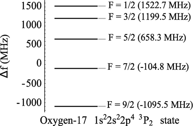
Figure 1:The hyperfine structure of the ground state of oxygen-17. The hyperfine levels are shown with respect to the center of gravity of the ground state
Adding together nuclear spin, represented by the quantum number I, and the total electronic angular momentum, represented by the quantum number J, results in a new angular momentum vector that we call the total angular momentum of the atom, represented by the quantum number F. Hyperfine structure generally has a much smaller energy splitting compared to fine structure. Like every angular momentum vector we have encountered, the F vector can also point in different orientations. For example, an state has four possible orientations described by the quantum numbers 3/2, 1/2, 1/2, and 3/2. All four of those orientations have the same energy.
Compatibility with Energy
We often care about what observables are compatible with energy. At the end of Chap. 7. Angular Momentum, we used the ket to represent the states of the hydrogen atom (one electron). All the different quantum numbers in this ket represent observables that are compatible with energy.
Important Reminder
The observables represented by and are not compatible energy.
Let’s update our ket with information we have learned from this chapter. When we add together nuclear spin and total electronic angular momentum, the cones representing those angular momenta are tilted with respect to the total atomic angular momentum (F). Just like when we added orbital and electron spin, the cone heights of I and J, which are represented by the quantum numbers and , are no longer compatible with energy. Therefore, our new ket is .
The nucleus of a hydrogen atom has a nuclear spin represented by . The atomic ground state of hydrogen has the electronic configuration , or , , and . Because the nucleus has spin, there will be two hyperfine levels represented by () and (, 0, and 1). Therefore, the four hyperfine levels for the ground state have kets:
The three hyperfine levels with are degenerate and have the same energy. The hyperfine level with has a different energy.
So, the ground state of hydrogen has two hyperfine levels represented by the quantum numbers and . For something a bit more complicated, let’s look at the ground state of europium. Europium has 7 electrons in its last, unfilled subshell. All isotopes of europium have a ground state term symbol , or (), , and . If europium had no nuclear spin, that would be the end of the story. We would define the ground state:
to have 0 energy. However, both stable isotopes of europium have nuclear spin: europium-151 (63 electrons, 63 protons, 88 neutrons, and ) and europium-153 (63 electrons, 63 protons, 90 neutrons, and ). Other isotopes of europium will have different nuclear spin. For example, europium-152, which is radioactive with a half-life of 13.5 years, has a nuclear spin quantum number of . Each of these europium isotopes have hyperfine levels.
Summary
If an isotope has no nuclear spin, there would be 1 ground state. If it does have nuclear spin, there are multiple ground states. This is because the angular momentum from the nucleus exerts a torque on the electrons, which results in a small splitting and shift of the state’s energy.
There is a single exception to the above summary that we will discuss more in Sect. 9.2 Math. If the state has no total electronic angular momentum (), there is still only a single state; the single state does not split into multiple hyperfine levels. However, that single state will still have an F quantum number as a label.
9.2 Math
We can find the possible values of F by using the largest to smallest in integer steps rule. The rule is:
Let’s do a few examples.
Example 1
Hydrogen-1 has a nuclear spin quantum number of and the ground state has a total electronic angular momentum quantum number of (also since hydrogen has a single electron). Therefore, the possible F values for the ground state range from to in integer steps. Thus, there are 2 hyperfine levels for the ground state of hydrogen-1.
Example 2
Oxygen-17 has a nuclear spin quantum number of and the ground state has a total electronic angular momentum quantum number of . Therefore, the possible F values for the ground state range from to in integer steps. Thus, there are 5 hyperfine levels for the ground state of oxygen-17. Those values, which are shown in Fig. Figure 1, are 9/2, 7/2, 5/2, 3/2, and 1/2.
Example 3
Let’s consider the two stable isotopes of europium: europium-151 and europium-153. Both stable isotopes of europium have the same nuclear spin quantum number of . The ground state has a total electronic angular momentum quantum number of . Therefore, the possible values for F range from to in integer steps, resulting in 6, 5, 4, 3, 2, or 1.
Quick Quiz
The radioactive isotope europium-152 has a nuclear spin quantum number of . How many hyperfine levels will the ground state have, and what are their F quantum numbers?
Beryllium-9 has a nuclear spin quantum number of with a ground state total electronic angular momentum quantum number of . How many hyperfine levels will the ground state have, and what are their F quantum numbers? The answers are below the maze shown in Fig. Figure 2.

Figure 2:A fun maze to separate the quiz from the answers
The answers are:
7 levels: 13/2, 11/2, 9/2, 7/2, 5/2, 3/2, or 1/2
1 level: 3/2.
Notice that beryllium-9 still has a single ground state even though the nucleus has spin. This is because , so the range of possible F values is 3/2 to 3/2. This always happens when . However, the nucleus still has angular momentum, so we include in the description of the state.
Using quantum mechanics, we can derive the energy splitting of a hyperfine level with respect to the center of gravity:
where A is called the magnetic dipole hyperfine constant and B is called the electric quadrupole hyperfine constant. Notice that everything else in the above equation apart from A and B is a quantum number. Theorists can calculate the hyperfine constants A and B while experimentalists measure them. When we perform spectroscopy on an atom with hyperfine structure, we can measure the energy spacing between all of the hyperfine levels and use the above equation to back out experimental values of A and B. Some hyperfine constants were measured many years ago while others have yet to be measured. For example, the ground state hyperfine constants for europium-151 and europium-153 were measured for the first-time way back in 1960 by P.G.H. Sandars and G.K. Woodgate and published in the journal Proceedings of the Royal Society A.[1] Sandars and Woodgate found that the magnetic dipole hyperfine constant and the electric quadrupole hyperfine constant for the ground state of europium-151 is MHz and MHz. To convert those numbers into energy, just plug the hyperfine constants into the above equation and multiply the result by Planck’s constant, h. If someone already measured those numbers, we can use those as a starting point for our fitting algorithms. If not, we have to determine them ourselves.
For every state in an atom, the electrons have different quantum numbers. States with higher n tend to be farther from the nucleus while the angular momentum quantum numbers represent different orbitals. Therefore, for an atom with nuclear spin, every state in that atom will have different hyperfine constants resulting in a different hyperfine splitting. Even the same state in two different isotopes that happen to have the same nuclear spin will have different hyperfine constants because the nuclei of the two isotopes are slightly different.
Summary
The “splitting” of the center of gravity into hyperfine levels is described by Eq. (5). The magnetic dipole hyperfine constant A is zero unless both and . The magnetic quadrupole hyperfine constant B is zero unless both and .
One Final Thing
The magnetic dipole term (the term with A) in Eq. (5) tends to be larger than the electric quadrupole term (the term with B). For example, the ground hyperfine state of europium-151 has a splitting . The first term in parentheses is from the magnetic dipole term and the second is from electric quadrupole term. There are additional terms to Eq. (5), but they are very small compared to the electric quadrupole term. The next term in the formula is the magnetic octupole term, which contains quantum numbers and the magnetic octupole hyperfine constant C. This term is generally unnecessary unless you have exceptionally good data. The magnetic octupole constant is zero unless both and .
9.3 Transition Frequencies
Suppose we have an atom with a nuclear spin quantum number of . To help distinguish between the lower and upper states, we will use primes on the quantum numbers for the excited states. In this example, the lower state has a total angular momentum quantum number of and the upper state has . Our goal is to write an equation for the transition frequency between two hyperfine levels. We first need to find the possible values for F, which can range from to in integer steps, giving and . Since as well, the possible values for are and , see Fig. Figure 3. In this hypothetical example, the hyperfine level has a smaller energy than the hyperfine level while the order is reversed in the excited state; the ordering of the quantum number all depends upon the interaction with the nucleus.
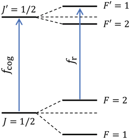
Figure 3:A simple Grotrian diagram for a made-up atom
Next, we want to find the transition frequency from the hyperfine level to the hyperfine level. Using Eq. (5), we can calculate the hyperfine energy splitting. We will use “LS” for lower state and “US” for upper state. Note that since and , both and . Evaluating Eq. (5) with the given quantum numbers, we find and . According to Fig. Figure 3, the state has more energy than the center of gravity for the lower level, meaning . Since , we also learn that . For the upper state, the hyperfine energy splitting is also positive. For this state, the formula is , which implies that in order to make .
Quick Quiz
Suppose an electron in our made up atom is in the lower hyperfine level. What is the formula to calculate the transition frequency from the lower hyperfine level to the upper hyperfine level? Your answer should contain the center of gravity frequency and the two magnetic dipole hyperfine constants and . The answer is in the footnotes.[2]
The general formula to calculate the transition frequency between two hyperfine levels is
For many learners, the signs of the shifts can be confusing, so let’s explore the signs with our toy example. Let’s start with the minus sign in front of . According to Fig. Figure 3, the hyperfine state reduces the transition frequency compared to . Since for that state, the minus sign makes sense. What about if we wanted the transition frequency from the lower hyperfine level? For that state, , so that minus sign turns into a plus sign, increasing the frequency needed compared to . This is a subtle but important point, so take some time to convince yourself the transition frequency from any lower hyperfine level to any upper hyperfine level is given by Eq. (6). Using this same logic, convince yourself that the plus sign in front of makes sense.
9.4 Example with Cesium-133
Figure Figure 4 shows a spectrum from a paper we published in 2018,[3] in which we performed saturated absorption spectroscopy on cesium-133. Cesium-133 has a nuclear spin quantum number of . The first five shells of cesium are completely filled, leaving a single electron in the 6s subshell. The ground state has the term symbol while the excited state has a term symbol . So, the ground state has two hyperfine levels, and , while the excited state has four hyperfine levels, 2, 3, 4, and 5. The and ground hyperfine levels are well separated from each other (9.192 GHz), which is much larger than the Doppler width for transitions from either state. Therefore, we will not have any crossovers despite having two lower states.
![Experimental spectroscopic results of the transition in neutral cesium-133. This is an experimental result from my research group, see reference [1]. A simplified Grotrian diagram for the transition can be found in Fig.](/AtomicPhysicsForEveryone/build/541577_1_En_9_Fig4_H-ed805ecf26588984819f3ea339e51032.png)
Figure 4:Experimental spectroscopic results of the transition in neutral cesium-133. This is an experimental result from my research group, see reference [1]. A simplified Grotrian diagram for the transition can be found in Fig. Figure 12
We performed spectroscopy from the ground hyperfine level, which has an energy approximately 4.021 GHz above the center of gravity for the ground state. Given The Rule (Eq. (18)) , 0, or 1 with the exception , we can excite an atom from the ground state hyperfine level with to the excited state hyperfine levels with 3, 4, or 5.[4] Each of these three real transitions has a Lorentzian lineshape. We also have three V crossovers. For a review of crossovers, see Chap. 5. Saturated Absorption Spectroscopy, Sect. 5.2 Crossovers. The first crossover comes from the two real transitions and . We often write this crossover in shorthand form: . The other two crossovers are the and crossovers. Despite having 6 spectroscopic features, the frequencies of all 6 features depend on only five parameters: the two hyperfine constants for the ground state, the two hyperfine constants for the excited state, and the transition frequency between the center of gravity for the ground state and the center of gravity for the excited state, see Eq. (6). I should point out that the width and amplitude of each peak are also free parameters, but we didn’t really care about those. Our main goal was to measure the center of gravity frequency and the hyperfine constants. Having 5 parameters to determine the position of all spectroscopic features is typical. The experimental data from our group on a transition in europium-151 had up to 77 spectral features in that spectrum![5] Even still, the center of each feature is determined by only 5 free parameters.
Let’s apply Eq. (6) using numbers from cesium-133. The spectrum in Fig. Figure 4 is from the , ground state. The excited state has and 3, 4, and 5.[6] Let’s find for all of the features.
9.4.1 Real Transitions
There are three real transitions in the spectrum. They are
Let’s calculate the shift from the center of gravity for the state for each real transition. Since these are shifts for the excited state, we will use the primed values in Eq. (5). We will also need Eq. (6) to find the transition frequency between two hyperfine levels. Since the hyperfine splitting for the ground state is so large, we will perform our spectroscopy with respect to the ground hyperfine level. For ease of reference, here are those equations:
where is the frequency of light needed to go from the ground hyperfine level to the center of gravity of the state. I also replaced the quantum numbers with primed values and the hyperfine constants with “US” subscripts.
Let’s do the math for the real transition. First, let’s find K:
Now we can find the hyperfine splitting for the state from the center of gravity for the state.
Table Paragraph shows the results of the math. The hyperfine constants for the state are kept as unknowns that we find while fitting the data. If there weren’t any crossovers, we would be done. Our fitting function would be the sum of three Lorentzian functions[7] whose centers are taken from the above table:
Table 9.2 The energy shifts for the hyperfine levels with respect to the center of gravity for the state in cesium-133. All of the real transitions in this example are from the ground hyperfine level
| Transitions | ||
|---|---|---|
where is the frequency of light needed to go from the ground hyperfine level to the center of gravity of the state. To avoid accidentally mixing up the magnetic dipole hyperfine constant of the state and the amplitude of the Lorentzian functions, I changed the variable for amplitude to C. If we wanted to write the transition frequencies in terms of the actual center of gravity frequency, we would replace with .
9.4.2 Crossover Transitions
For this spectrum, there are three V crossovers: , , and . The center of the spectral feature due to the crossover is found using the same procedures we learned about in Chap. 5. Saturated Absorption Spectroscopy, which is adding the two real transitions and dividing by 2:
The same procedure can be done for the other two crossovers. In the end, the fit function is a sum of 6 Lorentzian functions. From the fit, we find , , and , all with uncertainty. You will get to practice this in a homework problem.
9.5 Optional: Amplitudes
A common question I am asked is if there is a way to calculate the amplitudes of the Lorentzian functions. Finding the absolute amplitude is possible, but quite difficult. However, if the spectral features aren’t overlapping (we often use the phrase “well-separated features”), we can find the relative amplitudes for the real transitions. It uses a mathematical symbol you may not have seen before, but you should think of it as a placeholder for a lot of hidden algebra. Not many people do the hidden algebra themselves—that’s what Mathematica is for—but if you search the internet for “Wigner 6-j,” you can find all the math behind the symbol. The scaled amplitudes of the real transitions are given by the following formula:
where the primed quantum numbers are for the excited state. That last symbol is called the Wigner 6-j symbol (it is squared in the above equation). Also, the second element of the second row is the number 1 (lots of folks accidentally read that as the nuclear spin quantum number I). In Mathematica, you would type SixJSymbol[{J,I,F},{Fp,1,Jp}] (Mathematica doesn’t allow J’ or F’ as variable names, so I replaced them with Jp and Fp). There are also online calculators you can find by searching the internet for “Wigner 6-j symbol calculator”. Notice this formula has no units. We use this formula to take ratios to find relative amplitudes.
Let’s find for all three real transitions in the cesium-133 example we have been studying. To make things a bit easier, I included a copy of Fig. Figure 4 on this page. As a reminder, the ground state has quantum numbers and , the excited state has and , and the nuclear spin is .
From this math we see that the is the largest transition. Using this largest transition as the reference, we can compare the size of the other two transitions to it. The transition, which is the peak around 5 MHz in Fig. Figure 5, is times smaller than the transition. Finally, the transition is times smaller than the transition. If you look at the amplitudes of the real transitions, you’ll see that these estimates are pretty close to what was measured experimentally.
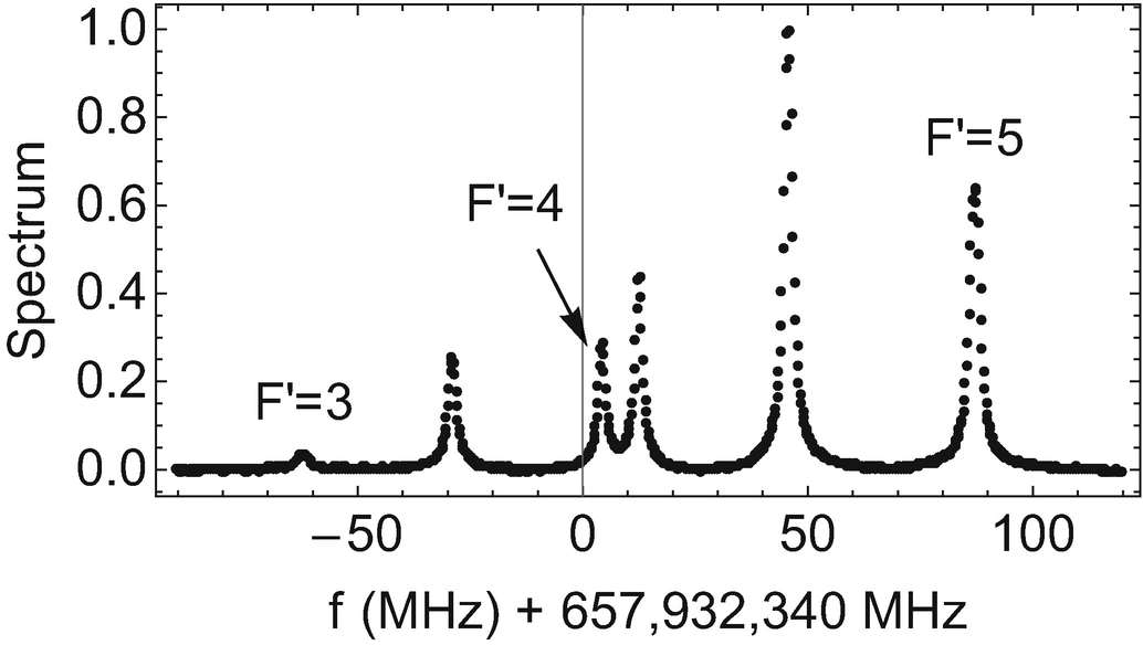
Figure 5:Experimental spectroscopic results of the transition in neutral cesium-133. This is an experimental result from my research group. A simplified Grotrian diagram for the transition can be found in Fig. Figure 12
While it is possible to calculate the amplitudes of the crossovers, it is much more complicated. One reason is that the number of atoms with a particular velocity, which creates the crossovers, depends on the temperature of your vapor cell. However, we at least have a fairly straightforward way of finding the relative amplitudes of the real transitions.
9.6 Example with Oxygen-16
Oxygen-16 has no nuclear spin, so there is no hyperfine structure. Shortest section ever!
9.7 Example with Oxygen-17
Oxygen-17 has a nuclear spin quantum number of , so there will be hyperfine structure. Below is a table of the seven lowest energy states for atomic oxygen.
Table 9.3
| Electron configuration | Term symbol | Energy () | f (Hz) |
|---|---|---|---|
| 0 | |||
| 158.265 | |||
| 226.977 | |||
| 15,867.862 | |||
| 33,792.583 | |||
| 73,768.200 | |||
| 76,794.978 |
For oxygen isotopes with no nuclear spin, such as oxygen-16, this table provides all the information about their atomic states. There is a single ground state with electronic configuration and term symbol . However, due to hyperfine structure, the table does not tell the whole story for oxygen-17. Let’s examine the ground state of oxygen-17. For this state, the total electronic angular momentum quantum number is and the nuclear spin quantum number is . The possible values for the total atomic angular momentum quantum number are:
We can also calculate the energy splitting using the hyperfine splitting formula. For convenience, here is the hyperfine splitting formula:
The first thing to notice is that for the ground state, both and , so we will need both the magnetic dipole term (the term with A) and the electric quadrupole term (the term with B). For example, the hyperfine splitting for the hyperfine level is:
where and are the hyperfine constants for the ground state. Each energy level in the above table will have different hyperfine constants.
Next, let’s explore the state, which has an energy of above the ground state and a total electronic angular momentum quantum number of . Using the rule to find F, we find a single possible value: . This only happens when a state has quantum number . With the constraint , we find
Even though the nucleus has angular momentum, there is no energy shift when . This hyperfine level has the same energy as the center of gravity. However, we will still label this state with the F quantum number: . You will explore the hyperfine structure of oxygen-17 more in Problem Exercise 9.3.
9.8 Problems
References
Williams, W.D., Herd, M.T., Hawkins W.B.: Spectroscopic Study of the and States in Cesium-133. Laser Phys. Lett. 15(9), 095702 (2018). https://
doi .org /10 .1088 /1612 -202X /aac97 Sandars P.G.H., Woodgate G.K.: Hyperfine structure in the ground state of the stable isotopes of europium. Proc. R. Soc. Lond. A. 257, 269–276 (1960). Sandars & Woodgate (1960)
Maruko, C., Cölmek, N., Herd, M.T., Ahrendsen, K., Cabrales, B., Cannon, G., Davis, E., Guo, X., Karani, T., Wallace, A., Wisnauckas, K., Williams, W.D.: Spectroscopic study of the transitions in neutral europium-151 and europium-153: absolute frequency and hyperfine structure. J. Opt. Soc. Am. B. 41, 1217–1223 (2024). Maruko et al. (2024)
Herd, M.T., Maruko, C., Herzog, M.M., Brand, A., Cannon, G., Duah, B., Hollin, N., Karani, T., Wallace, A., Whitmore, M., Williams, W.D.: Spectroscopic study of the transition in neutral europium-151 and europium-153: absolute frequency and hyperfine structure. J. Opt. Soc. Am. B. 39, 2596–2602 (2022). Herd et al. (2022)
How cool of a journal name is that?! See reference [2] for the full citation.
.
Reference [1].
A full list of the rules that need to be satisfied for an electron to transition between two atomic states is given in Appendix C. Transition Rules.
See Reference [4] for the full citation.
There is also an excited hyperfine level, but we cannot excite an atom from the ground hyperfine level to this state.
There are many subtleties that we are glossing over here. Spectra sometimes have an offset, a sloped offset, or a Gaussian pedestal for various reasons. When you fit data, sometimes you have to add something to your fit function. However, you should always have a reason for why you are adding something to your fit function.
Ground state citation: Reference [2]. and citation: Reference [3]. citation: Reference [4].
You should, of course, do an internet search for “parity physics” if you’d like to learn more.
- Sandars, P. G. H., & Woodgate, G. K. (1960). Hyperfine structure in the ground state of the stable isotopes of europium. Proceedings of the Royal Society of London. Series A. Mathematical and Physical Sciences, 257(1289), 269–276. 10.1098/rspa.1960.0149
- Maruko, C., Çölmek, N. N., Herd, M. T., Ahrendsen, K. J., Cabrales, B., Cannon, G., Davis, E., Guo, X. Y., Karani, T., Wallace, A., Wisnauckas, K., & Williams, W. D. (2024). Spectroscopic study of the 4f 7 6s 2 8 S 7/2∘ – 4f 7 ( 8 S ° ) 6s6p( 1 P ° ) 8 P 5/2,7/2 transitions in neutral europium-151 and europium-153: absolute frequency and hyperfine structure. Journal of the Optical Society of America B, 41(5), 1217. 10.1364/josab.521181
- Herd, M. T., Maruko, C., Herzog, M. M., Brand, A., Cannon, G., Duah, B., Hollin, N., Karani, T., Wallace, A., Whitmore, M., & Williams, W. D. (2022). Spectroscopic study of the 4 f 7 6 s 2 8 S 7/2∘−4 f 7 ( 8 S ∘ )6 s 6 p ( 1 P ∘ ) 8 P 9/2 transition in neutral europium-151 and europium-153: absolute frequency and hyperfine structure. Journal of the Optical Society of America B, 39(10), 2596. 10.1364/josab.467968