One-dimensional wave mechanics
Learning objectives
After this chapter, you should be able to:
solve the time-independent Schrödinger equation in regions of constant potential;
impose boundary and matching conditions;
distinguish bound states from scattering states;
calculate spectra and wavefunctions for the infinite square well;
use probability current to interpret reflection and transmission;
explain tunneling through a classically forbidden region; and
describe the harmonic oscillator with ladder operators.
Sections 7.1–7.6 form a core progression from boundary-value problems to probability flow and tunneling. The above-barrier resonance subsection is an optional extension. Section 7.7 introduces a second solution strategy—the oscillator’s algebraic ladder method—and can be taught after the well and current sections without requiring the resonance extension.
7.1 Schrödinger’s equation in position space
Chapter 6 developed the position representation in the abstract: operators become differential expressions, and a ket becomes a wavefunction. This chapter puts that machinery to work on the simplest possible setting, a single spatial dimension, where boundary conditions and matching conditions turn into concrete, solvable calculations. For one nonrelativistic particle of mass in a potential ,
If is time independent, a separated solution obeys
This is an eigenvalue equation for the Hamiltonian. A normalizable energy eigenfunction changes only by an overall phase, so its probability density is stationary.
The local behavior of a solution depends entirely on the sign of :
if , solutions oscillate with ;
if , solutions grow or decay exponentially with ; and
at abrupt finite changes in , both and are continuous.
The last condition follows by integrating the differential equation across an arbitrarily narrow interval: a finite jump in cannot produce a -function in , so cannot jump either. Infinite potentials are the one exception, and it is worth being precise about why. An infinite wall forces at the wall, but is allowed to jump there, because the argument just given assumed a finite jump in . An infinitely deep well is really the limit of an ever-taller finite well, not a literal potential one can integrate across.
Physically, equation (2) is nothing more than the same eigenvalue problem introduced abstractly in Chapter 3, specialized to the position representation of Chapter 6. acting on becomes a second-order differential operator acting on . Nothing new is being postulated here—only the concrete form that an old postulate takes once a continuous basis is chosen.
7.2 The infinite square well
This is the simplest bound-state problem in quantum mechanics, and it is worth solving completely: every later matching calculation in this chapter repeats the same basic steps on a harder potential. Let for and elsewhere. The wavefunction vanishes at and . Inside,
The first boundary gives ; the second requires . Thus
and
Boundary conditions have quantized the energy. There is no state: it would be the zero function and could not be normalized. The nonzero ground-state energy is required by confinement and the uncertainty principle—a state squeezed into a region of size cannot also have , so it cannot have .
The infinite well is the simplest model of confinement, and its qualitative lessons reappear whenever a particle is trapped: quantum dots, particles in optical lattices, and nucleons in a schematic nuclear well are all discussed using the same vocabulary of quantized levels and a nonzero ground-state energy. One more pattern is worth noting now, because it will recur for every bound-state problem in this chapter: the integer counts the number of interior nodes of . More nodes means more curvature, and more curvature means higher energy, since curvature is exactly what converts potential energy into kinetic energy in equation (2).
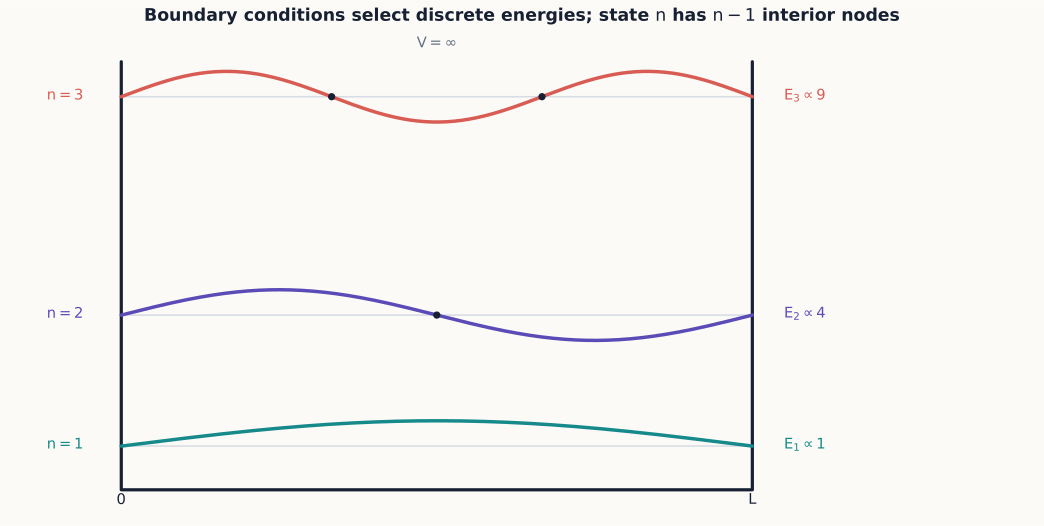
Figure 1:Hard-wall boundary conditions admit only wavelengths that fit the box. Higher brings both more nodes and more curvature, so the kinetic energy rises as rather than in equal steps.
Example 7.1: a superposition in the well
Suppose
Then
The energy probabilities stay , but the position density contains an interference term proportional to . A superposition of stationary states need not itself have a stationary density.
Concept check 7.1
Why is called stationary if it depends on time?
Answer
Its time dependence is an overall phase, so and every time-independent observable distribution are constant.
7.3 General bound states
A bound state is normalizable and localized. For potentials approaching constants at infinity, bound-state energies lie below the asymptotic potential, so the wavefunction decays exponentially outside the classically allowed region.
Several qualitative facts are useful before solving anything further:
one-dimensional bound-state energies are nondegenerate;
the ground state has no interior nodes;
higher states have successively more nodes; and
for an even potential, eigenstates can be chosen with even or odd parity.
The nondegeneracy claim deserves a moment’s justification, and it is special to one dimension specifically. Two independent solutions of a second-order ordinary differential equation at the same would be related by their Wronskian. Normalizability at both infinities forces that Wronskian to vanish, which in turn forces the two solutions to be proportional to one another—so there is really only one independent bound state at that energy. Chapter 8 will show that this argument fails in three dimensions, where rotational symmetry routinely produces several independent states at one energy.
The finite square well
For a finite square well, oscillatory interior solutions must be matched to decaying exterior solutions. The matching conditions produce transcendental equations rather than the simple integer rule of the infinite well. The finite well has only finitely many bound states, and each leaks into the classically forbidden region.
Let for and for , with . Inside, the wavefunction oscillates with ; outside, it decays with . Because the well is symmetric about , every bound state can be chosen even or odd, and it is enough to match at and use the symmetry to fix the other boundary automatically. Matching and gives
Neither equation can be solved in closed form, but both are constrained by energy conservation, , which is independent of . In terms of the dimensionless variables and , this constraint is the quarter circle
and the bound states are exactly the intersections of this circle with the curves (even) and (odd) in the first quadrant. The dimensionless number measures the well’s “strength”: how many oscillations the interior wavefunction can complete before decay must take over.
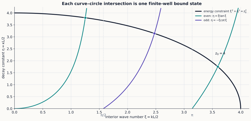
Figure 2:For , the constraint circle meets two even branches and one odd branch. Enlarging the circle admits another state only after it crosses the next branch threshold.
This picture, without any further algebra, already answers the two questions that matter most:
A one-dimensional well always binds at least one state. As , , so the even branch always starts at the origin and rises to meet the circle of any radius . However shallow or narrow the well, there is always exactly one even, nodeless bound state. This is a genuinely one-dimensional fact; shallow three-dimensional wells can fail to bind anything at all.
New states appear at regular intervals of . The tangent branch diverges at and the cotangent branch changes sign there, so a new branch of the even curve enters the first quadrant every time passes a multiple of , and a new branch of the odd curve enters every time passes an odd multiple of . The total bound-state count, for , is therefore
At an exact threshold the prospective new solution has and is not normalizable, so it does not yet count as a bound state; this is why the ceiling formula, rather than “floor plus one,” handles threshold values correctly. Away from exact thresholds the two forms agree. The states alternate even, odd, even, odd, as grows. Only once do the lowest levels approach the -spaced infinite-well energies of equation (5); the topmost bound state, barely below , always looks qualitatively different—loosely bound with a long decaying tail.
Example 7.2: counting bound states
Take a well with . Since , , and , the value has passed the first two thresholds but not the third: one even branch exists from , a second even branch appears once , and one odd branch appears once , while the second odd branch (threshold ) has not yet appeared. Equation (11) confirms this directly: . This well supports exactly three bound states: two even and one odd.
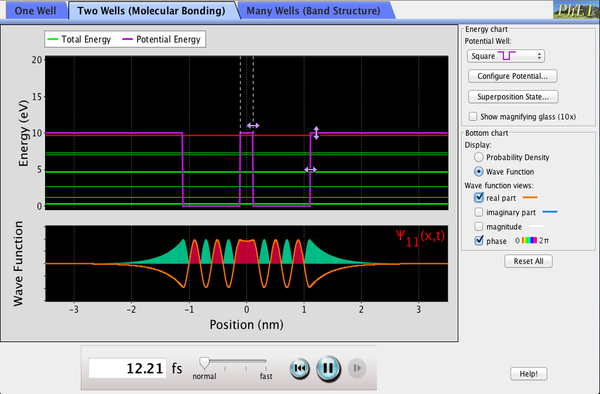
Figure 3:Set up a finite well and drag its width and depth to change , watching bound states appear at the thresholds equation (11) predicts. The same sim’s other potential shapes carry forward to the harmonic oscillator later in this chapter and to the variational estimates of Chapter 10.
Interactive simulation: Bound States
Concept check 7.2
Does a shallow, narrow finite well always fail to bind a particle if is small enough?
Answer
No. Equation (11) gives for every : a one-dimensional attractive well of any strength binds at least one even, nodeless state. Only in higher dimensions can an arbitrarily weak well fail to bind anything.
7.4 Probability current
Scattering problems ask how probability flows, not merely how large a wave-amplitude coefficient is. Equation (1) implies the continuity equation
where
For , . Reflection and transmission probabilities are therefore ratios of outgoing to incoming current. This velocity weighting is essential when two regions have different wave numbers, as the step problem shows next.
7.5 Scattering from a step
Bound states are only half the story: a particle with enough energy to escape to infinity produces a scattering state instead, and the relevant questions become “how much reflects?” and “how much transmits?” rather than “what are the allowed energies?” Consider a particle incident from the left on
For , write
where and . Matching and at gives
Even though , reflection occurs because the wavelength changes abruptly. The amplitude is not by itself the transmission probability when the speeds differ. Using the current from Section 7.4 gives
Probability conservation plays the role here that particle-number bookkeeping played in Stern–Gerlach chains.
Concept check 7.3
Can a particle reflect from an upward step when ?
Answer
Yes. Matching waves of different wavelengths produces a reflected amplitude. Classical certainty of transmission is not the quantum prediction.
Total reflection below the step
Now suppose . Region II no longer oscillates. Boundedness as , together with the absence of an exponentially growing incoming term from the right, leaves the purely decaying solution , with . Matching and at as before gives
Both numerator and denominator have the same magnitude , so exactly: every particle reflects, exactly as a classical particle would. What is not classical is that is nonzero. The wavefunction penetrates into the classically forbidden region with an exponentially decaying tail, even though the probability current carried by a purely real exponential vanishes identically,
since and differ only by the real factor . The forbidden region has nonzero probability density but carries no net probability flow toward , consistent with . This statement does not assign a trajectory in which an individual particle travels in and then returns.
Writing in polar form exposes a reflection phase shift with no classical analog. If (an infinitely high step, i.e. an infinite wall), : the familiar node-forcing hard-wall reflection. For finite , the phase interpolates continuously between this hard-wall value and as —which matches the formula for evaluated at , so the two regimes join smoothly at threshold even though their functional forms look unrelated.
Example 7.3: how a soft wall differs from a hard one
For (a step exactly twice the particle’s kinetic energy), equation (18) gives . The reflection probability is still , but differs by a quarter cycle from the hard-wall answer . A detector counting reflected atoms cannot see this phase directly; an interference experiment that recombines the reflected wave with another coherent path can.
Concept check 7.4
For at a step, is the probability density zero in the classically forbidden region?
Answer
No. is nonzero and decays smoothly. What vanishes is the probability current there, so no probability permanently escapes to ; is still exact.
7.6 Tunneling through a barrier
Section 7.5 showed total reflection when for a step that stays high forever. What changes if the classically forbidden region has finite width instead? Let a rectangular barrier have height and width . Inside the barrier, solutions are exponential rather than oscillatory, yet matching at both boundaries leaves a nonzero transmitted amplitude. The exact transmission probability is
For a thick or high barrier, ,
The exponential dependence explains why tunneling is highly sensitive to barrier width and particle mass. Tunneling does not mean the particle borrows energy and violates conservation. An energy measurement in the stationary scattering state still gives ; the spatial wavefunction simply extends through a region where a classical particle of that energy could not travel.
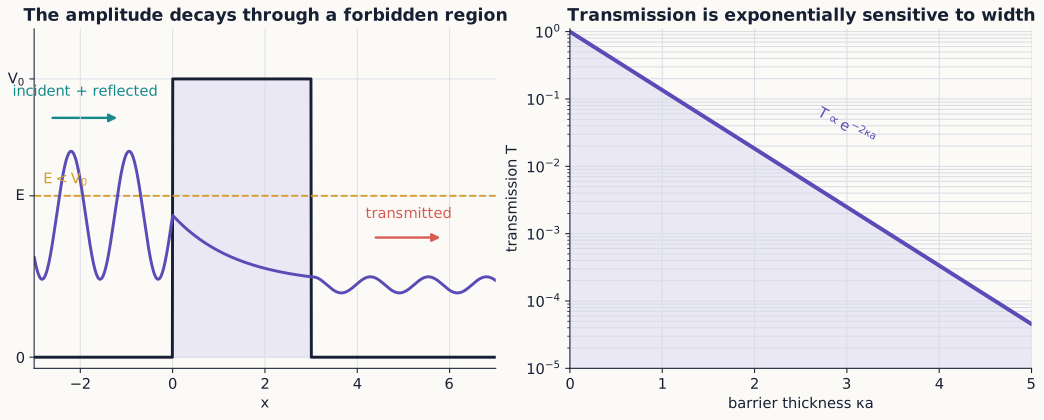
Figure 4:Inside a classically forbidden barrier the stationary wavefunction is exponential, not absent. Matching it at the second boundary leaves a transmitted amplitude whose probability is extraordinarily sensitive to barrier width.
Example 7.4: compare two barrier widths
In the thick-barrier regime, increasing by multiplies by . If , the transmission falls by . This sensitivity underlies scanning tunneling microscopy and many decay processes.
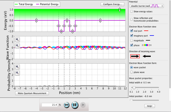
Figure 5:Send a wave packet at a rectangular barrier and adjust its width and height to see the exponential sensitivity of equation (20) directly: a reflected packet, a smaller transmitted one, and no borrowed energy anywhere. A CheerpJ simulation takes tens of seconds to load on a cold cache and is mouse-only.
Interactive simulation: Quantum Tunneling
Optional extension: above-barrier resonant transmission
Equation (20) was derived for , but the same matching calculation applies for , where the interior solution oscillates instead of decaying, with . Formally replacing —so that —turns equation (20) into
Unlike the tunneling regime, this transmission is not monotonic in the barrier width. Whenever for an integer —the barrier width equals a whole number of half wavelengths of the interior wave— and : the barrier becomes completely transparent, exactly as an antireflection coating of the right thickness eliminates reflected light. Away from these resonances, some reflection persists even though classically guarantees transmission. The two formulas meet consistently at , where both and vanish and a careful limit of either expression gives the finite value rather than an ambiguous .
Concept check 7.5
If a barrier is thick enough that , can it ever be perfectly transparent?
Answer
Not for : grows without bound, so only shrinks with increasing width. Perfect transmission () is a feature of the resonant regime in equation (22), where the interior wave oscillates rather than decays.
7.7 The harmonic oscillator
Every bound state so far was found by directly solving a differential equation and matching boundary conditions—a fresh calculation for each new energy level. The harmonic oscillator admits a much slicker, purely algebraic route that sidesteps this repetition entirely. For
define
They satisfy , and
The spectrum does not follow merely by naming these operators, so here is the essential argument. Define . For every normalized state,
so its eigenvalues cannot be negative. The commutator above gives
Therefore raises any energy eigenvalue by , while lowers it by the same amount. Starting from a number eigenstate with eigenvalue , repeated lowering would produce . Because number eigenvalues cannot be negative, this sequence must terminate at a state annihilated by . For that state, , so its number eigenvalue is zero. The original must therefore have been a nonnegative integer. Repeated raising gives every , and the norms of the raised and lowered states fix the ladder factors:
with
The ground state is defined by . In position space this first-order equation gives a Gaussian, as Example 7.5 works out explicitly. The ladder method obtains the complete spectrum without solving a new differential equation for every level: every excited state is reached from by repeated algebra with , rather than by solving a new second-order boundary-value problem for each as the earlier well problems required.
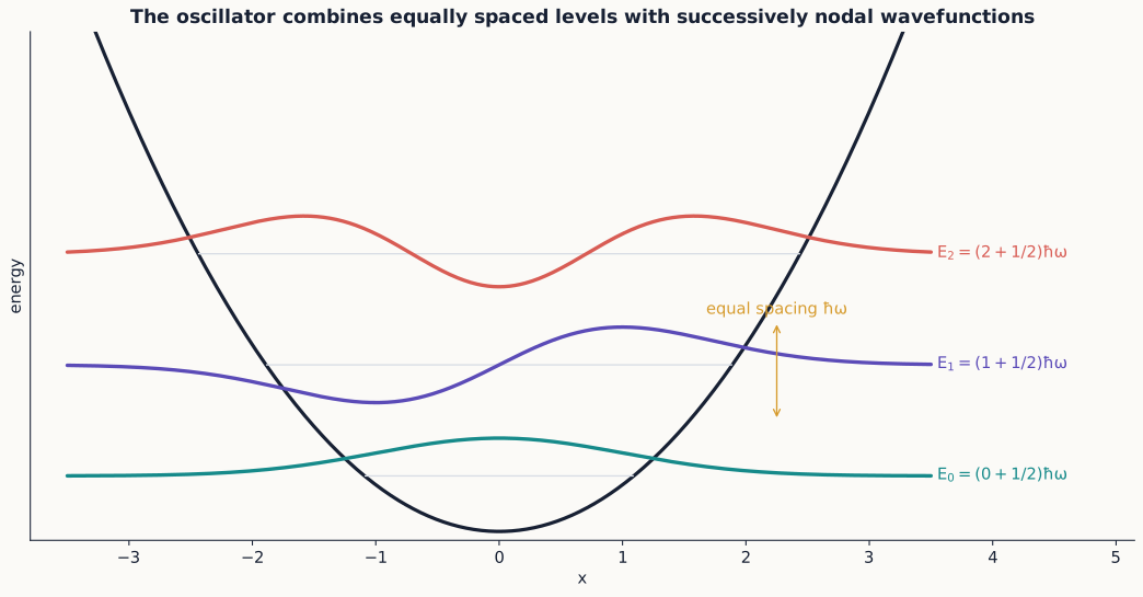
Figure 6:Unlike the square well, the oscillator has equal energy spacing. The ladder operator raises both the energy by and the node count by one, building every state from the Gaussian ground state.
Example 7.5: the ground state in position space
Writing , the condition becomes the first-order equation
Integrating and normalizing gives
This is a Gaussian of exactly the form studied in Chapter 6 as a minimum-uncertainty wave packet, with width and zero mean momentum. It therefore saturates , just like the minimum-uncertainty packets of that chapter. But this particular Gaussian does not spread with time the way a free-particle packet does: it is an exact energy eigenstate, so is stationary. Confining harmonic forces, unlike free propagation, can hold a minimum-uncertainty packet in a permanent balance between spreading and restoring force.
Concept check 7.6
Why does the oscillator not have ?
Answer
The ground state has . A state with both zero kinetic and zero potential energy would require exact and , contradicting .
Summary
Stationary wavefunctions solve a Hamiltonian boundary-value problem.
Confinement produces discrete energies and a nonzero ground-state energy.
A finite well always binds at least one state, and gains new states at regular intervals of its dimensionless strength .
Scattering probabilities are ratios of probability currents; total reflection below a step can still carry a nonclassical phase shift and a nonzero forbidden-region density.
Wavefunctions can penetrate forbidden regions and tunnel through finite barriers without violating energy conservation, while the same matching calculation above a barrier predicts resonant, perfectly transparent energies.
Ladder operators reveal the equally spaced harmonic-oscillator spectrum and generate every excited state algebraically from one Gaussian ground state.
Exercises
Exercises 1–12 form the core set on wells, probability flow, tunneling, and the oscillator algebra. Exercises 13–19 deepen boundary matching and below-step reflection. Exercises 20–24 are synthesis or optional-extension problems.
Find for every infinite-well energy eigenstate by symmetry.
For , calculate explicitly and identify its oscillation period.
Show that no two distinct normalizable bound states in one dimension can have the same energy by analyzing their Wronskian.
Derive and for the potential step and verify equation (17).
Calculate the current for .
Derive the continuity equation from the Schrödinger equation and its complex conjugate.
Estimate the change in thick-barrier transmission when the particle mass is multiplied by four.
Verify from .
Derive equation (25).
Show that has energy .
Example 7.5 derives the ground state . Apply to in position space to find explicitly, and verify by direct substitution that it solves equation (2) with .
Boundary-matching consolidation
Starting from continuity of and at , and using the symmetry of the well to relate to , derive the even- parity condition in equation (8).
Derive the odd-parity condition in equation (9) following the same steps as Exercise 13.
For a well with , find the total number of bound states and how many are even and how many are odd.
Explain, using the limit of , why a one-dimensional finite well can never have zero bound states, no matter how small or is.
Derive equation (18) by matching and at for .
Show directly from equation (18) that for every , and confirm that as .
Show that the probability current vanishes identically for , for any constant , and explain why this is consistent with .
Extensions and synthesis
Derive equation (22) from equation (20) by the substitution , and find the smallest barrier width giving for a given .
Take the limit of equation (20) carefully (expanding ) to show that , and check that the same value follows from equation (22) in the limit .
Using the Gaussian ground state of equation (31), calculate and explicitly and confirm .
Explain, in terms of Ehrenfest’s theorem from Chapter 6, why the mean position of an oscillator energy eigenstate is time independent even though a classical particle of the same energy oscillates back and forth.
Compare the ground-state energy of the harmonic oscillator with the ground-state energy of an infinite well of width (a rough width match). Which is larger, and why might that be expected from the shape of the two potentials near their minima?
Selected exercise guidance
Use these checks only after making a complete attempt.
Exercise 5
Use separately for the incident, reflected, and transmitted traveling waves. The reflected current points left, so uses its magnitude. Substituting the matched amplitudes should give .
Exercise 8
Because , multiplying the mass by four doubles . In the thick-barrier approximation the exponent therefore changes from to , apart from the algebraic prefactor.
Exercise 15
. The parity alternates from the even ground state, so there are three even states and two odd states.