Position and momentum representations
Learning objectives
After this chapter, you should be able to:
interpret a wavefunction as the coordinates of a state in a continuous basis;
normalize wavefunctions and calculate position probabilities;
represent position and momentum operators in coordinate space;
transform between position and momentum representations;
use commutators to derive translations and uncertainty bounds; and
calculate expectation values for continuous observables.
Sections 6.1–6.7 form the conceptual core. Sections 6.8–6.9 are applications to packet spreading and expectation-value dynamics; they may be taken as a second pass before the chapter’s final representation check.
6.1 From discrete labels to a continuum
Every chapter so far has worked with a spin’s discrete state space: two basis kets, a handful of amplitudes, sums instead of integrals. A particle’s position, by contrast, can take a continuum of values, and this chapter extends the same logic that worked for spin to that continuous setting. Spin states already taught us the key idea: a ket is abstract, and a column of numbers is only its representation in some chosen basis. Position simply uses a basis with a continuous label instead of a discrete one. The generalized ket represents an ideal position outcome, and the position-space wavefunction is defined exactly as an amplitude was for spin:
The completeness relation, which for spin was a finite sum over two basis kets, becomes an integral over the continuum of possible positions:
so that
The basis is delta-normalized:
The Dirac delta is not an ordinary finite function; it is defined entirely by its effect inside an integral:
One consequence follows immediately: ideal position kets are not normalizable physical states at all. Real preparations are wave packets of finite width, as Section 6.5 develops in detail.
Optional mathematical detail: why the delta is singular
It helps to see directly why an ordinary finite function cannot play the role of , rather than simply asserting it. Suppose instead that for some bounded function . Completeness would then require
to equal for every state . But a bounded kernel convolves and smooths a function as it integrates against it; it cannot reproduce the function’s exact value at a single point. The only way it could would be for the kernel to be concentrated entirely at with unit weight there, and no ordinary function is simultaneously concentrated at one point and normalized to integrate to one. Only the singular limit of an infinitely narrow, infinitely tall spike—the Dirac delta—has the sifting property we actually need. This is the same logic that made a discrete basis’s Kronecker delta work for spin: orthonormality is exactly what lets us read off a coefficient by taking an inner product. The continuum version of that same requirement forces delta-function normalization in place of unit inner products, and it is exactly what pushes the generalized kets just outside the space of normalizable states.
6.2 The continuous Born rule
The probability of finding the particle between and is
Normalization requires
Unlike a discrete probability, is a probability density, with units of inverse length. This has a striking consequence: the probability of finding the particle at any one exact point is zero, even at a point where the density itself is nonzero.
This is a genuine conceptual shift from the spin chapters, not merely a change of notation. There, was already, by itself, a probability. Here one more step—multiplying by an interval , or integrating over a finite range—is required before a number between 0 and 1 appears. Forgetting this step is the most common bookkeeping error when moving from discrete to continuous quantum mechanics: a “large” value of at some point says only that a narrow interval there carries appreciable probability, not that the point itself is likely.
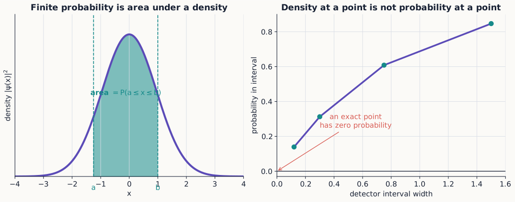
Figure 1:In a continuous measurement, height is a density and area is probability. Shrinking the detector interval to zero removes its area even when the density at the selected point remains nonzero.
Example 6.1: normalize an exponential packet
Let with . Because makes the integrand symmetric about the origin, the integral over the whole line splits into twice the integral over , where and the exponential is easy to integrate directly:
so one convenient choice is . For , the integrand is an odd function times an even one, hence odd overall, and an odd function integrated over a range symmetric about the origin always integrates to zero; so without any further calculation. For , the same even/odd split as before applies, and the standard integral (obtained by integrating by parts twice, or by differentiating twice with respect to ) gives
Thus .
Concept check 6.1
Is the probability that a position measurement gives exactly ?
Answer
No. It is a density. A finite probability requires integration over a finite interval, and the density carries units of inverse length.
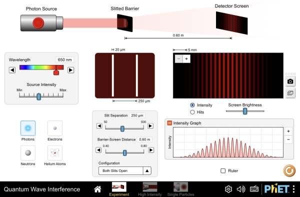
Figure 2:Send electrons, photons, or atoms one at a time through a double slit and watch each arrive as a single dot, yet build up the interference pattern predicted by over many trials. Cover one slit with a detector and the pattern collapses to two bands, the continuous-variable version of Chapter 1’s Rule 3.
Interactive simulation: Quantum Wave Interference
6.3 Operators in the position representation
Position acts by multiplication:
Momentum acts by differentiation:
Apply both operator orders explicitly to an arbitrary function , rather than taking the commutator below on faith. The term first differentiates, then multiplies by :
The term first multiplies by , then differentiates the product using the ordinary product rule:
Subtracting, the term proportional to —the piece generated by the derivative landing on itself—is identical in both orderings and cancels exactly, leaving only the extra term the product rule generates when the derivative instead lands on the factor of :
Since was an arbitrary function, this is an operator identity, true independent of any particular state:
The expectation values are
Boundary behavior matters here in a way it did not for spin.
Quick calculation: integration by parts and the boundary term
Hermiticity of would require for every pair of states . Writing the left side as an integral and integrating by parts once,
The remaining integral on the right is exactly , the quantity symmetry of requires the left side to equal. Thus the two sides agree when the boundary form vanishes for every pair in the operator’s domain. Square integrability alone does not guarantee a pointwise limit at infinity; one also needs suitable regularity and boundary behavior. The standard momentum domain on the whole line is chosen so these conditions hold.
An unbounded operator is therefore not fully defined by a differential expression alone: its domain is part of its definition. A further subtlety appears on a finite interval. Requiring wavefunctions to vanish at two hard walls makes the boundary form vanish, so is symmetric on that domain, but it is not self-adjoint there and does not define the well’s momentum observable. The operator with the hard-wall boundary conditions does define a self-adjoint Hamiltonian. Chapter 7 uses that Hamiltonian directly.
Concept check 6.2
If is multiplied by the constant phase , do or change?
Answer
No. The phase cancels from all expectation values. A position-dependent phase, such as , can change momentum statistics.
Example 6.2: phase carries mean momentum
That last remark is worth demonstrating explicitly, since it is easy to mistake “the phase doesn’t matter” for a blanket statement rather than one about constant phase specifically. Let , where is real, normalized, and vanishes at infinity. Then
because . The density does not reveal at all; only the spatial phase carries that information. As in the spin interferometer of Chapter 4, phase information becomes observable only through a suitable measurement.
6.4 Momentum states and Fourier transforms
Momentum eigenstates satisfy . In position space,
The momentum-space wavefunction is
with inverse
These are basis changes, not dynamical evolution: exactly the same distinction Chapter 2 drew between rewriting a spin ket in a new basis and performing an actual measurement. Normalization is preserved either way: .
A broad packet in position generally requires a narrow range of wave numbers; a narrow position packet requires many. This Fourier fact underlies the position–momentum uncertainty relation, and separating what is and is not quantum here matters. As a mathematical statement about pairs of Fourier partners, it has no quantum content of its own: it is true of classical wave pulses too. What quantum mechanics adds is the physical claim that , not merely , is a genuine probability amplitude for an equally real, independently measurable observable. A classical wave packet’s Fourier width is a statement about its mathematical shape; a quantum wavefunction’s Fourier width is simultaneously a statement about the distribution of a different physical quantity’s measured values.
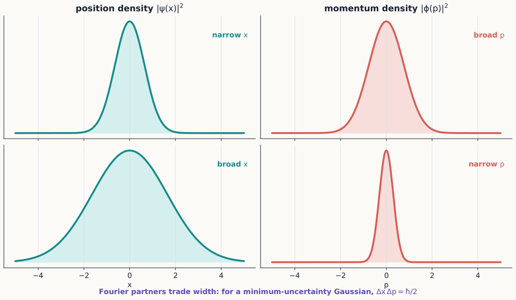
Figure 3:Position and momentum descriptions are Fourier partners. Localizing the same state more tightly in one representation necessarily spreads it across more basis states in the other.
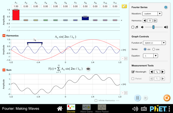
Figure 4:Add harmonics one at a time and watch a broad range of wave numbers synthesize a narrow, localized packet in position, or remove harmonics and watch the reverse. The spread displayed for each domain is exactly the trade-off behind equation (27) below.
Interactive simulation: Fourier: Making Waves
Concept check 6.3
Does a momentum eigenfunction describe a localized physical particle?
Answer
No. Its magnitude is constant over all space and it cannot be normalized in the ordinary sense. It is a generalized basis state; physical beams are modeled by normalizable superpositions with a range of momenta.
6.5 Gaussian wave packets
A normalized Gaussian centered at with mean wave number can be written
It has
Thus
The Gaussian saturates the Robertson bound associated with equation (17). This uncertainty is not, however, caused by a badly calibrated position detector kicking the particle around. It describes the spreads found in two genuinely different ensembles, each prepared identically in the same state, one measured for position and the other for momentum.
Optional mathematical extension: why the Gaussian saturates the bound
For the canonical pair, equality in the Cauchy–Schwarz argument behind the uncertainty relation can occur only when the two centered state vectors are related by
for some real number . It is worth solving this condition explicitly for , , to see directly why the minimizing states turn out to be Gaussian and not some other shape. In the position representation, with momentarily set to zero for simplicity,
a first-order differential equation with solution
Normalizability requires the exponent to decay, so must be negative; writing reproduces exactly the Gaussian profile of equation (25) (restoring simply reinserts the phase , which affects neither nor ). No other line shape solves equation (28): any state that is not Gaussian must have strictly. So Gaussian wave packets, far from being merely a convenient textbook example, are the states of least joint position–momentum uncertainty: there is no better one to be found.
Example 6.3: overlap of two wave packets
How distinguishable are two Gaussian packets prepared with the same width and mean wave number , but different centers and ? Their overlap is
where the common phase has canceled between and . Writing , the identity separates the exponent into a piece that integrates to the normalization and a piece that depends only on the separation:
Packets separated by many widths () are nearly orthogonal and behave as reliably distinguishable preparations; packets separated by less than a width overlap substantially, and no measurement can sort individual particles between them with certainty. This is the continuous counterpart of the Stern–Gerlach statement that only exactly orthogonal spin states are perfectly distinguishable: here “exactly orthogonal” is replaced by “infinitely far apart,” and any finite separation always leaves some residual overlap.
Concept check 6.4
Two Gaussian packets of width are centered apart. Are they reliably distinguishable by an ideal position measurement?
Answer
Yes, to excellent approximation. Equation (32) gives an overlap of , so the two states are nearly orthogonal and a position measurement almost always lands cleanly in the region associated with the correct packet.
6.6 Momentum generates translations
Define the translation operator
Using , the exponent becomes , so in the position representation the exponential’s defining power series—the same construction reviewed in Chapter 4 for a matrix exponential, now applied to the differentiation operator instead—gives
This is exactly the Taylor series of expanded about the point , so
The translated packet is centered a distance to the right: its value at equals the old packet’s value at . Infinitesimally,
Momentum is therefore the generator of spatial translations, just as the Hamiltonian is the generator of time translations and spin components generate rotations. The pattern is always the same: a Hermitian observable exponentiates into a unitary operator that implements a continuous symmetry, and the observable’s expectation value is conserved exactly when that symmetry leaves the Hamiltonian unchanged. Chapter 9 will show that orbital and spin angular momentum generate rotations in precisely this sense, so that the rotation operators already used for spin in Chapter 4 are a special case of a single unifying structure that also produces (33) here.
Conjugating position by the translation gives
This operator statement makes the geometry independent of any particular wavefunction: it is true for every state at once, not just the ones we happen to write down explicitly.
Concept check 6.5
Does translating a state by change the magnitude of its momentum-space wavefunction?
Answer
No. Since commutes with , translation multiplies by the pure phase and leaves unchanged. Sliding a packet in space redistributes nothing among its momentum components; only where it is found changes, not how fast it is found to be moving.
6.7 Measurement resolution and wave packets
An ideal sharp position measurement uses projectors only as a mathematical limit. A detector pixel covering a region corresponds instead to
Selecting that detector outcome produces a state localized to the region, after normalization. A narrower region generally broadens the momentum distribution. This is the continuous version of an analyzer preparing an outcome state, with finite detector resolution replacing an ideal one-dimensional projector.
6.8 Application: free-particle evolution and packet spreading
For , each momentum component is an energy eigenstate with . The momentum wavefunction evolves as
Its magnitude is unchanged, so the momentum distribution stays fixed for all time. The phase, however, is nonlinear in , and transforming back to position shows that this nonlinear phase causes a packet to spread. For the minimum-uncertainty Gaussian of equation (25),
The center, meanwhile, moves classically:
A narrow initial packet spreads faster than a broad one, because a narrow packet in position necessarily contains a broader range of momenta—and therefore a broader range of velocities—than a broad one does.
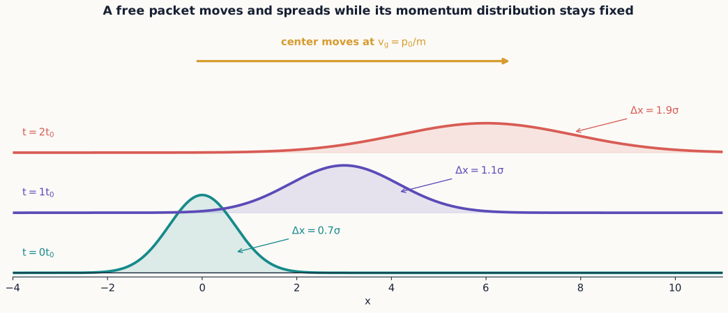
Figure 5:Free evolution advances the packet center at the group velocity while its constituent momentum components separate. The fixed momentum spread therefore appears as a growing position spread.
Group and phase velocity
A plane-wave component has phase velocity , while the packet envelope itself travels at the different speed
It is the group velocity that matches the particle’s classical velocity. Confusing the two gives a factor-of-two error for the nonrelativistic dispersion relation . The phase velocity is not meaningless—it governs how the fine ripples inside the envelope move—but it is not what a particle detector downstream registers as “how fast the particle arrived.” For a narrow-band packet, the carrier oscillations do not appear separately in , whereas the envelope locates the probability packet. Its group velocity is therefore the speed to compare with the packet’s classical motion.
6.9 Application: Ehrenfest’s theorem
For
the expectation-value equation from Chapter 4 gives
These resemble Hamilton’s equations, and it is tempting to conclude that quantum expectation values always follow classical trajectories. They do not, in general: except in special cases. The center of a narrow packet in a slowly varying potential only approximately follows a classical trajectory.
There is one important exception, and the reason it arises deserves a closer look. For quadratic potentials, the equations close exactly for the means. The reason is purely algebraic: the discrepancy is controlled by the higher moments of , through a Taylor expansion of about . Every term in that expansion beyond the first involves at least , or a higher power still. If is linear in —equivalently, if is at most quadratic—that Taylor expansion has no higher terms at all, and the mean-value equations close exactly, regardless of how wide the packet is. For any other potential, this gap is generally nonzero and grows with the packet’s spread.
Ehrenfest’s theorem does not turn a quantum state into a classical point. The packet retains its uncertainties, may spread, and may even split into reflected and transmitted pieces. Classical behavior emerges only for suitable states, observables, potentials, and time scales, not as a general guarantee.
Example 6.4: constant force
For , equation (44) gives
The mean follows the classical constant-acceleration trajectory exactly, even though the position distribution need not remain narrow.
Example 6.5: the harmonic oscillator
For , studied in full in Chapter 7, is linear, so equation (44) closes exactly:
Differentiating the first equation and substituting the second gives
the classical simple-harmonic equation of motion, satisfied exactly by and for any initial state—a narrow packet, a broad one, or a superposition of many energy eigenstates. Together with Example 6.4, this shows that exactly classical mean motion is not a generic feature of quantum dynamics; it is a special consequence of having a potential no steeper than quadratic. The width of the packet is a separate question entirely: for the free particle it grows without bound (equation (40)), while a harmonic packet prepared in the right shape returns periodically to its initial width, oscillating in step with .
Concept check 6.6
For the harmonic oscillator, does Ehrenfest’s theorem guarantee that a widely spread-out state behaves like a classical particle in every respect?
Answer
No. It guarantees only that the means and trace the exact classical trajectory. The state can remain highly uncertain, and observables other than these first moments—such as itself—need not follow any classical law.
6.10 A representation is not a physical location
In momentum space the same abstract operators act differently:
Nothing has happened to the particle when one changes from to . One has simply changed the basis used to describe the same ket. A physical position measurement, by contrast, changes conditional predictions through state update. This distinction is the continuous analog of rewriting a spin ket in the basis versus actually sending it through an analyzer.
Summary
A wavefunction is a state’s coordinate function in the position basis.
Squared wavefunction magnitude is a probability density.
Position multiplies by , while momentum differentiates in the position representation.
Position and momentum wavefunctions are Fourier transforms of one another.
Gaussian packets attain the minimum uncertainty product and, apart from their center, mean momentum, and overall phase, are the unique states that do so.
Momentum generates translations, connecting symmetry with observables; the same pattern reappears for time evolution and rotations.
Ehrenfest’s theorem closes exactly only when the potential is at most quadratic; otherwise it describes an approximate classical trajectory for the mean.
Finite-resolution measurements project onto ranges rather than exact points.
Exercises
Exercises 1–12 build the core representation, normalization, Fourier, and translation skills. Exercises 13–17 accompany the dynamics applications. Exercises 18–34 are deeper derivations and synthesis; a first course should select from them rather than assign the entire bank at once.
Normalize on and zero elsewhere. Find and .
For the exponential packet in Example 6.1, find the probability that .
Verify equation (17) by applying both operator orders to an arbitrary differentiable function.
Show by integration by parts that is real when vanishes at infinity.
Normalize on and zero elsewhere.
Find for a real, normalized wavefunction that vanishes at the boundaries of its domain.
Verify the four moments stated for equation (25).
Fourier transform a Gaussian by completing the square and confirm .
Show that and that .
Derive to first order in using the commutator.
A detector reports only whether or . Write its two projectors and the conditional wavefunction after the result.
Explain how two wavefunctions can have identical position densities but different momentum distributions. Give an explicit pair.
Dynamics applications
Derive equation (40) by evolving the Gaussian in momentum space, or verify its short- and long-time limits.
Find the time at which the width of a free Gaussian has doubled.
Derive both Ehrenfest equations using commutators.
Give a potential for which for every state and one for which it is generally false.
Verify the momentum-space representation of by differentiating the Fourier kernel.
Further extensions and synthesis
Suppose for a bounded function with . Show that generally differs from for a wavefunction that varies on the scale over which is spread, and explain why only the Dirac-delta limit removes this discrepancy for every .
Using equation (32), find the separation , in units of , at which .
Repeat the overlap calculation of Example 6.3 for two Gaussian packets with the same center but different mean wave numbers , and show that the result depends on and in a way that parallels equation (32).
Solve equation (28) for , keeping general from the start, and confirm that the phase appears with .
Verify by direct substitution that the harmonic-oscillator Ehrenfest equations of Example 6.5 combine to .
Identify the mathematical feature shared by the free particle and the harmonic oscillator that allows Ehrenfest’s theorem to close exactly for both, and explain why a cubic potential does not share it.
A particle is confined with certainty to a finite interval . Explain using the Fourier relation why its momentum-space wavefunction cannot be concentrated at a single value of .
Verify and for the Gaussian packet of equation (25) by direct integration, and confirm the stated and .
Two Gaussian packets share a center but have different widths and . Compute their overlap and show that it depends only on the ratio .
Show that a momentum eigenstate is unchanged in magnitude, up to an overall phase, under any translation , and interpret this as the statement that momentum eigenstates carry no distinguishing spatial location.
Show directly from its integral definition that in Section 6.7 is Hermitian and idempotent ().
Model a detector pixel of width centered at by . Show that as , recovering the probability density from a finite-resolution measurement.
Find the time at which for a free Gaussian packet, in terms of , , and .
Compute the group velocity for the relativistic dispersion relation , and show that it reduces to when .
A student measures momentum, obtains a result, and then asks for the “position-space picture” of the resulting state by Fourier transforming. Explain what has and has not been physically established about position by this point, contrasting it with an actual position measurement.
A real, even wavefunction satisfies . Using the Fourier relation between and , show that is real and even, and use that fact to show without evaluating the momentum integral directly.
Prove that is unitary directly from its exponential definition and the Hermiticity of .