Composite systems and entanglement
Learning objectives
After this chapter, you should be able to:
construct product states and operators with tensor products;
calculate joint, marginal, and conditional probabilities;
distinguish separable states from entangled states, including in mixtures;
use reduced density operators to describe a subsystem;
predict correlations in Bell states and quantify partial entanglement with the Schmidt decomposition;
explain why entanglement does not enable faster-than-light signaling;
state the Tsirelson bound and what it does and does not imply about nature; and
analyze simple two-qubit gates and measurement protocols.
Sections 5.1–5.6 provide the core route: build joint states, calculate local and joint predictions, interpret Bell correlations, and create entanglement. Section 5.7 is an optional quantitative extension using the Schmidt decomposition. Section 5.8 begins with the essential distinction between correlation and entanglement, then marks its Werner-state test as an advanced extension.
5.1 Building a joint state space
Chapters 2 through 4 developed a complete quantum description of a single spin: a two-dimensional complex state space, Hermitian operators for measurable quantities, and unitary time evolution. But that formalism, on its own, does not say how to describe two spins that were prepared together and are later measured separately, perhaps in two different laboratories. A first guess might be that each spin simply carries its own independent ket, and a joint experiment just reports the two kets’ separate predictions side by side. That guess is sometimes right and sometimes badly wrong, and sorting out the difference is the subject of this chapter.
The correct joint state space is built from the two one-spin spaces by a specific mathematical construction called the tensor product. It is not merely “the two spaces considered together”: it is a larger space, big enough to hold every possible correlation between the two spins, including correlations with no classical counterpart at all. Learning to build this space, and learning to recognize when a joint state does or does not reduce to “two independent spins,” is the first step toward composite systems of any size—two electrons, a spin coupled to a field mode, or the many-particle systems of Chapter 11.
One spin- system has a two-dimensional state space. Two distinguishable spins require four independent basis states:
The joint space is the tensor product . We abbreviate as or, for qubits, . In the ordered basis,
If and , then
Notice that the coefficient array factors into one list for and one for . This factorization is the defining feature of a pure product state, and it is exactly what will fail, in Section 5.2, for a state that cannot be built this way.
Quick calculation: multiplying out a concrete product state
Take and , so in the notation of equation (3), while and . Multiplying out term by term,
Only the terms ending in -label 0 survive, because has no component at all: the amplitude for any joint outcome with is forced to zero regardless of what does. Contrast this with the entangled state introduced next: here both surviving terms share the same label while ’s label is free to be either 0 or 1, exactly the signature of and having been prepared independently, with no correlation between their outcomes.
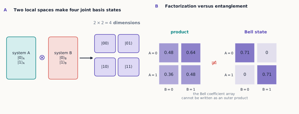
Figure 1:The tensor product expands two local two-state spaces into one four-state joint space. Product-state coefficients form an outer product of two local lists; the Bell-state pattern cannot be factored that way.
Operators on one subsystem
An operation on alone is represented by ; an operation on alone is . Operators acting on different subsystems always commute:
To construct these matrices rather than merely name them, replace every entry of the first matrix by that entry times the entire second matrix. For example, in the ordered basis ,
The first matrix flips ’s label while leaving ’s unchanged: and . The second multiplies a basis ket by the eigenvalue associated with ’s label while leaving alone. Multiplying these two explicit matrices in either order gives the same result, verifying the commutator above concretely. This block-matrix recipe is the Kronecker product used whenever subsystem operators must be written as a matrix on the joint space.
Because these operators commute, measurements made on the two distinct systems can always be assigned one common joint probability distribution, even when the individual components being measured on either spin, taken alone, would be incompatible. This is a stronger and more precise statement than just “the two measurements don’t interfere.” It says that a single joint probability distribution can be written down for the two experiments at all, which is exactly the kind of object that incompatible single-spin observables (Chapter 3) cannot generally be assigned to begin with.
Example 5.1: independent preparations
For , measurements of on both spins give and zero for the other outcomes. Since the preparation is a product, its joint probabilities factor:
Learning ’s result supplies no new information about . This factorization is the operational signature of a product state: every joint question about and can be answered by combining two separate one-spin calculations, and nothing is lost by treating the two laboratories as running independent experiments on a shared clock.
5.2 States that do not factor
Now consider the normalized state
Try to write it in the product form of equation (3). If while both and are nonzero, the required single-system coefficients contradict one another: there is no consistent choice of , , , that works. A state like this, which cannot be factored, is called entangled.
A joint measurement on produces 00 or 11, each with probability . Each individual outcome is random, yet the two records always agree. Rewriting the state in the basis gives
so the records also always agree. This is the key point: entanglement is not merely “both spins were prepared the same way.” No assignment of one definite pure state to each spin separately can reproduce all of these correlations at once.
The four Bell states form an orthonormal basis:
Relative signs that were invisible in a measurement become visible once we switch to another basis, exactly as relative phase did for a single spin in Chapter 2.
Being precise about what “entangled” means matters here, since the word invites an all-or-nothing reading it does not deserve. Entanglement is not a label attached loosely to “the two particles are correlated somehow”; it is a precise property of the joint state, and it comes in degrees. A state can fail to factor into a product yet still be much “closer” to a product than is. Section 5.7 makes this quantitative with the Schmidt decomposition. For now, treat the Bell states as one convenient orthonormal family of maximally entangled states, not as the only entangled states that exist.
Foundation check: factor or not?
Can be written as a product? What about ?
Answer
The first state factors as . The second does not: making the and coefficients nonzero while making both cross coefficients zero is impossible for a product of two one-qubit kets.
5.3 Joint, marginal, and conditional probabilities
For outcome kets and , the joint Born rule is
The marginal probability for ignores ’s result:
If is recorded, the conditional probability is when .
Example 5.2: joint, marginal, and conditional records
Begin with and measure both spins in the basis. Reading the four amplitudes directly gives
To ignore ’s record, sum across the two possibilities for :
Thus alone looks random. If is known, however,
so the same data are perfectly predictable after conditioning. Keep the three questions distinct: a joint probability concerns both records, a marginal deliberately ignores one record, and a conditional probability uses a known record to sort the trials.
The arbitrary-angle singlet formulas used in the Bell discussion are stated next. Their derivation is optional on a first pass.
Optional derivation: singlet analyzers at arbitrary angles
For the singlet
Measure along and along , and assign numerical results to the two outcomes. Chapter 3 gives the corresponding projectors as
The singlet density operator has the useful Pauli form
This identity can be checked by inserting the Pauli matrices and comparing the resulting matrix with . Now use the trace rules and . The joint Born rule gives
This calculation combines projectors, tensor products, density operators, and trace identities. It is an efficient derivation once those ingredients are familiar, but it should not be the first example used to learn the meaning of a marginal probability.
The resulting joint distribution is
and the correlation is
Aligned analyzers always disagree, perpendicular analyzers show no correlation, and oppositely aligned analyzers always agree, under these numerical labels. One more feature of equation (20) deserves a direct check: summing it over gives for every , independent of or . Each side’s own marginal statistics are, on their own, featureless coin flips. All the physical content lives in how the two records compare, not in either record alone—a point Section 5.4 develops further.
5.4 Reduced states
Suppose an experimenter has access only to spin , and never touches spin at all—perhaps has been carried off to a distant laboratory. What can that experimenter predict, given only the full joint state ? The answer is captured by the reduced density operator,
where the partial trace sums over any orthonormal basis of . Concretely, for any orthonormal basis ,
Each term is itself still an operator, but now acting on alone: ’s basis ket has been contracted away on both sides, and the sum over adds up the resulting -only pieces.
Let’s carry this out explicitly for , using the basis for . Writing out the full operator,
Tracing over means sandwiching this between and separately between , then adding the two results. Because while , any term whose two labels disagree vanishes immediately, including both off-diagonal terms, and , which are exactly the terms carrying ’s coherence. What survives is only
and the identical calculation, tracing over instead, gives as well.
Notice exactly which piece of information the partial trace discarded. It kept the diagonal terms, which correctly predict that a measurement of alone is 50–50. It discarded the off-diagonal coherence—the very feature that made a pure joint state rather than the classical mixture of Section 5.8. That coherence is a property of the joint operator alone; it has no counterpart living inside either local factor, which is exactly why no measurement confined to by itself can ever recover it.
The joint state is pure, but each subsystem, considered alone, is maximally mixed. This is not ordinary ignorance about which pre-existing Bell component actually occurred; the coherence that makes a pure state resides in joint off-diagonal terms such as , which the reduced state at alone cannot see.
If is measured in the basis and 0 is selected, is conditionally prepared in . If instead measures in the basis and selects , is conditionally prepared in . Yet before learning which setting was used, or what its outcome was, an observer at still assigns exactly , no matter what choice is made at .
This is a general feature, not a special property of : for any joint state, the reduced density operator used to predict ’s local statistics does not depend on which measurement, if any, is later performed at . Choosing a different analyzer at —or none at all—only changes how an already-fixed set of joint records can be sorted into subsets once the two sides compare notes; it cannot change the unconditional distribution of ’s own outcomes.
Here is the algebra behind that statement. If performs a complete projective measurement and the outcome is not supplied to , the joint state becomes
Taking the partial trace and cycling operators that act only on within that trace,
Completeness, , is the decisive step. The same result holds for any local operation at whose outcomes are pooled and whose probabilities sum to one. If one outcome is selected and communicated, however, uses a conditional state; that sorting requires the ordinary communication channel and cannot produce a signal before the message arrives.
Midpoint mastery check
Before moving to Bell inequalities, make sure you can do all four of the following without consulting the preceding pages:
expand a product ket in the four-state basis;
decide whether a pure two-qubit ket factors;
compute a joint probability and sum it to obtain a marginal; and
take a partial trace of a Bell-state density operator.
Diagnostic answers
A product expansion has coefficients . A pure coefficient array factors exactly when its coefficient matrix has determinant zero. Marginalizing means summing the joint probabilities over the ignored outcome. Tracing either half of any Bell state gives . If any of these steps is not yet routine, review Sections 5.1–5.4 before proceeding: the Bell and Schmidt calculations reuse all four skills.
Concept check 5.1
If , does that mean the spin at is definitely unpolarized and uncorrelated with ?
Answer
No. The reduced state fixes only ’s own unconditional statistics; it says nothing about whether ’s results agree, disagree, or vary independently with ’s. All four Bell states, the Werner state of Section 5.8 at every mixing parameter, and the classical mixture of Section 5.8 all give despite having very different—or no—correlations with . Correlation is a joint-state property; the reduced state has already thrown that information away.
5.5 Bell’s test of local hidden variables
A local hidden-variable model supposes that a measurement’s result is determined by information carried along from the shared source, and that a setting freely chosen at one station cannot affect the result recorded at a distant one. One experimentally useful constraint on any such model is the CHSH inequality. For two settings at and at , define
Every local hidden-variable model of this type satisfies .
The short argument makes several assumptions that should remain visible. The setting choices are statistically independent of the source variables (often called measurement independence); the result at either station does not depend on the distant setting (locality); and the recorded sample fairly represents the emitted pairs. Allowing a hidden-variable model to be stochastic rather than deterministic does not evade the bound: any local response probability can be treated as an average over additional local randomness, and averaging numbers that each lie between -2 and 2 cannot leave that interval. Real Bell experiments are designed to close setting, locality, and detection loopholes closely enough that these assumptions can be tested rather than silently presumed.
For the singlet, suitable coplanar settings separated by instead give . Quantum theory violates the classical bound while still preserving the no-signaling marginal probabilities from Section 5.4.
The conclusion this supports is precise, and it is worth stating carefully: the observed correlations cannot be reproduced by local models in which every result is fixed by shared pre-existing variables, independent of the later settings. Bell tests do not show that experimenters can send information backward in time or faster than light; Section 5.4 already ruled that out on its own.
The Tsirelson bound
Equation (28) shows that quantum mechanics can exceed the classical bound of 2, but it cannot exceed it arbitrarily. One can show that for the singlet, and more generally for any quantum state and any choice of -valued observables, . This number is the Tsirelson bound. The coplanar, -separated setting above is not a lucky combination that happens to violate the classical bound; it is the specific configuration that saturates the strongest violation quantum mechanics allows.
Why quantum mechanics stops at
Let be the four -valued observables and define the CHSH operator
Because each observable squares to the identity, direct multiplication gives
A observable cannot stretch a normalized vector by more than one, so each commutator has maximum stretch at most 2. Consequently has maximum stretch at most , and at most . Every expectation value therefore obeys . Suitable singlet analyzer directions reach the bound, so the inequality is tight rather than merely an estimate.
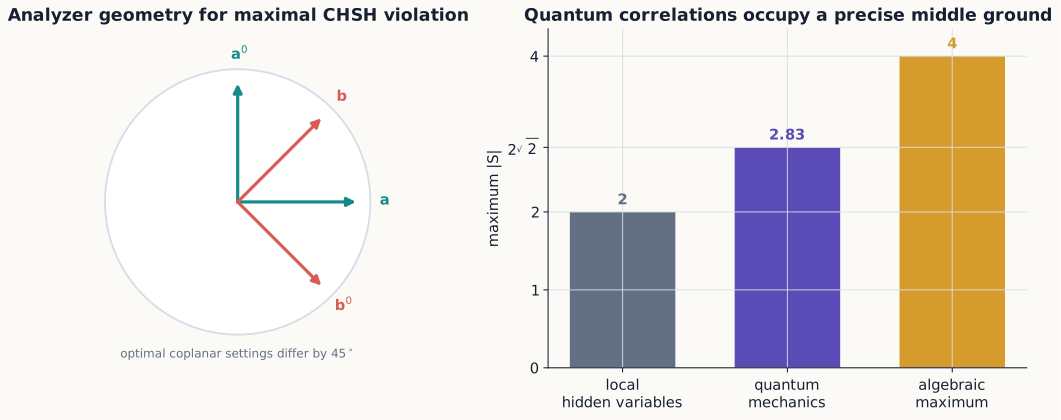
Figure 2:The optimal CHSH geometry places the two settings at each station between those at the other station. Quantum mechanics exceeds the local bound but stops well below the largest value that an arbitrary correlation table could produce.
Example 5.3: a setting that does not reveal a violation
A violation requires a specific relationship between the four analyzer directions; it does not happen automatically for any four directions we might pick. Suppose instead the four directions are chosen apart in sequence: , , , . Using from equation (21),
Here , well below even the classical bound of 2. The very same singlet, analyzed with a different—equally legitimate—choice of four directions, shows no sign of any nonclassical correlation at all. Demonstrating a Bell violation is therefore an experiment-design problem as much as a fact about the state: the directions must be chosen, as in the configuration above, to make the classical and quantum predictions disagree as sharply as possible. This is the same lesson Chapter 1 drew from sequential Stern–Gerlach analyzers: a single measurement rarely distinguishes rival explanations, and a well-chosen combination is needed to force them apart.
Concept check 5.2
Could a future theory find correlations stronger than quantum mechanics’s , while still forbidding faster-than-light signaling?
Answer
Logically, yes: no-signaling alone only forbids from being used to send a controllable message, and mathematical correlations (Popescu–Rohrlich boxes) exist that reach the algebraic maximum while keeping every local marginal exactly . Quantum mechanics happens to stop at . That intermediate value—more correlated than any classical local theory, less correlated than logical consistency alone would allow—is a specific, falsifiable feature of quantum theory, not a generic consequence of forbidding signaling.
5.6 Creating entanglement with gates
In quantum-information notation, the Hadamard gate is
and the controlled-NOT gate acts as . Starting from ,
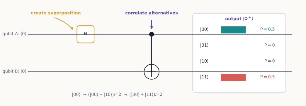
Figure 3:The Hadamard creates two coherent alternatives; CNOT correlates the second qubit with them. The output is still a pure state, but it is no longer a product of separate states for and .
The Hadamard creates a superposition in ; the controlled operation then correlates each alternative with a distinguishable state of . A reversible unitary process has produced a pure entangled state, with no measurement involved anywhere.
This last point deserves emphasis: entanglement is created by ordinary unitary evolution acting on a product input, just as a beam splitter followed by a phase shift can entangle two photons, or a spin–spin interaction term in a Hamiltonian can entangle two initially independent spins. Chapter 4’s rotations and this section’s entangling gates are the same kind of mathematical object—unitary operators—differing only in how many subsystems they act on jointly.
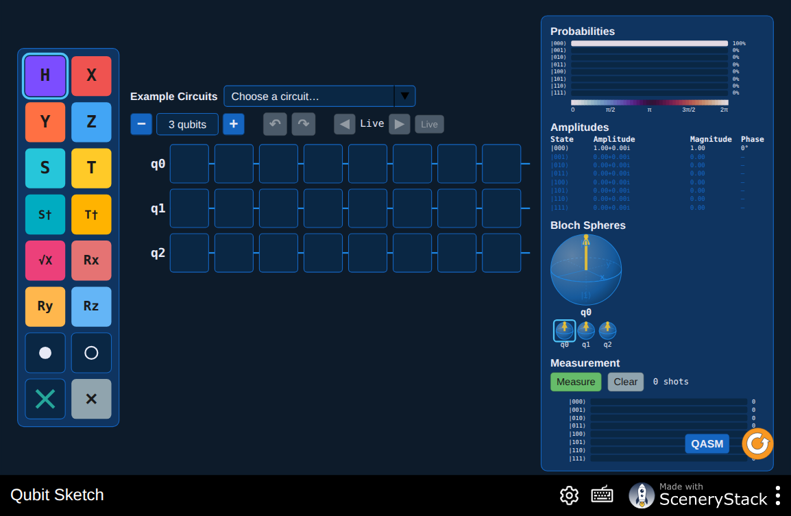
Figure 4:Drag a Hadamard gate onto qubit and a controlled-NOT between and to build the circuit above. Watch the two Bloch spheres and the joint-state amplitudes update live, and confirm that conditioning on ’s recorded result makes a definite prediction for a later measurement of , while ’s unconditional statistics remain unchanged.
Interactive simulation: Qubit Sketch
5.7 Optional extension: Schmidt decomposition and amount of entanglement
Section 5.2 promised a precise, quantitative way to say “how entangled” a state is. Every pure state of two finite systems can be expressed in suitable local orthonormal bases as
This is the Schmidt decomposition. The number of nonzero coefficients is the Schmidt rank. A pure state is a product exactly when ; it is entangled precisely when . The two reduced density operators share the same nonzero eigenvalues :
Worked method: finding a Schmidt decomposition
When a state is not already in Schmidt form, arrange its amplitudes as a coefficient matrix , with labeling rows and labeling columns:
Then . Its eigenvalues are the Schmidt weights , and its eigenvectors are the . The corresponding vectors can be recovered from
For example, consider a normalized state that is not visibly in Schmidt form,
The reduced state is
Its eigenvectors are and , with eigenvalues and . Applying the recovery formula gives the same two vectors on , so
This is the Schmidt decomposition. It immediately shows Schmidt rank two and therefore entanglement. In matrix language, the same procedure is the singular value decomposition of ; its singular values are .
For two qubits, the state
is already written in Schmidt form. At it is a product. At its coefficients are equal and each subsystem is maximally mixed: the fully entangled case.
A single number summarizing pure-state entanglement is the entropy of either reduced state:
It is zero for a product state and exactly one bit for a maximally entangled pair of qubits. For a pure joint state, this entropy measures entanglement by quantifying the mixedness of either reduced state. It is not, by itself, a general measure of all information or correlation in an arbitrary mixed state.
Example 5.4: a partially entangled state
Not every entangled state is maximally entangled. Take
already in Schmidt form with , (compare equation (34); this is the member of the family above). It does not factor: no choice of single-system amplitudes reproduces both nonzero coefficients while leaving the and coefficients zero, so the state is entangled. Its reduced state is
which has : alone is mixed, confirming the entanglement directly. Its entropy is
less than the 1 bit of a Bell state. So this state is entangled, verifiably so, and yet quantifiably “less entangled” than — exactly the kind of statement the all-or-nothing language of Section 5.2 could not make precise, but the Schmidt decomposition now can.
Example 5.5: conditional states in a rotated basis
Write as
The records always disagree, even though the and records always agree. Suppose obtains . Applying and normalizing leaves in . The joint state determines this conditional preparation exactly, while the outcome itself is still random. Changing basis reveals a different correlation pattern without changing the entangled state one bit.
5.8 Entanglement, mixtures, and correlation
Correlation alone does not prove entanglement; here is a clean example where it does not. The mixed state
has perfect agreement in , just like . But it lacks the off-diagonal coherence that made special. Rewriting in the basis shows that its outcomes are completely uncorrelated, whereas the Bell state remains perfectly correlated there too.
A mixed state is called separable if it can be written
Such states can still contain shared classical randomness, but nothing more. Entangled mixed states cannot be written this way. Bell-inequality violation certifies entanglement when it occurs, but some entangled mixed states do not violate any particular Bell test: the choice of measurement matters.
Optional advanced extension: the Werner-state boundary
A cleaner illustration of the boundary between separable and entangled is the Werner state,
a mixture of the maximally entangled with the maximally mixed two-qubit background , which carries no correlation at all. At this is two independent, fully random spins; at it is the pure Bell state. To locate the entanglement boundary rather than merely quote it, use the partial-transpose test. Transposing only changes a matrix element by
Every separable state remains positive under this operation. For two qubits, the converse also holds: a positive partial transpose is sufficient for separability. The partial transpose of has three eigenvalues and one eigenvalue . Adding the maximally mixed part therefore gives
The final eigenvalue becomes negative precisely when , certifying entanglement. For , all four eigenvalues are nonnegative and the two-qubit sufficiency result guarantees separability. Mixing in only a little of the entangled state therefore leaves a classically explicable mixture; only past a specific threshold does the joint state require entanglement. “How entangled” a mixed state is does not scale simply with how much of an entangled state was mixed in.
Curiously, the reduced state for every value of : local measurements at alone cannot distinguish any Werner state from any other, entangled or not. Whether is entangled is a fact about the joint state that no amount of data collected at alone, or at alone, can ever reveal.
Concept check 5.3
The reduced states of , , and every Werner state are all . Does this mean “entangled” is not a meaningful physical distinction, since it cannot be measured locally?
Answer
It means entanglement is a property of the joint state, not of either local marginal, so it cannot be certified from ’s data or ’s data considered separately. It remains an operationally meaningful and experimentally testable distinction: comparing the two players’ records after the fact—as in the CHSH statistic of Section 5.5, or the raw joint probabilities of Section 5.3—distinguishes them perfectly well. “Not locally measurable” is not the same as “not physically real”; it simply identifies which experiments are capable of detecting it.
Local unitary operations can rotate the Schmidt bases, but they cannot change the Schmidt coefficients, the reduced-state purity, or the entanglement entropy. Creating or destroying entanglement genuinely requires an interaction, a joint measurement, or discarding information into an external system; no amount of purely local fiddling will do it.
Concept check 5.4
Is entangled?
Answer
No. It factors as .
Concept check 5.5
For , does measuring create a random result at ?
Answer
The joint state already predicts correlated records. Conditioning on ’s record changes the state used for predictions at , but without that record ’s local results remain 50–50. No controllable local change identifies whether or how was measured.
Concept check 5.6
Can two different pure joint states have the same reduced state for ?
Answer
Yes. All four Bell states give . Local statistics do not contain all information in a joint state.
Summary
Composite state spaces are tensor products, and their dimensions multiply.
Product states factor into subsystem states; entangled states do not.
Joint probabilities can contain perfect correlations while each marginal distribution remains random.
A partial trace gives the state relevant to local measurements.
Bell correlations violate a bound obeyed by local hidden-variable models but do not permit faster-than-light signaling, and quantum mechanics itself never exceeds the Tsirelson bound .
Superposition followed by a controlled gate can create entanglement.
Entanglement is quantitative, not binary: Schmidt coefficients and entanglement entropy measure how far a state is from a product, and mixed states such as the Werner state are entangled only above a threshold mixing parameter.
Exercises
Exercises 1–12 are the foundational set. Exercises 13–18 consolidate the core ideas and begin using the optional Schmidt machinery. Exercises 19–32 are extensions and synthesis problems; assigning a representative subset is more useful than treating all fourteen as routine end-of-chapter practice.
Core practice
Expand in the joint basis.
Determine which states factor: , , and .
Calculate all joint probabilities for each Bell state.
Rewrite in the basis and describe its correlations.
For the singlet, use equation (20) with an angle of to find all four joint probabilities.
Compute and the entanglement entropy for . Is pure?
Show that a product pure state has a pure reduced density operator.
Prove from equation (20) that both local marginal distributions are for every pair of settings.
Use singlet correlations to evaluate the CHSH expression for directions with planar angles .
Write the matrix of CNOT in the ordered computational basis and verify its action on all four basis kets.
Start with each computational basis state, apply Hadamard to and then CNOT, and identify the resulting Bell state.
Explain why the phrase “each entangled spin has a definite but unknown state” fails for when both and correlations are considered.
Find the reduced density operators and entanglement entropy of .
Verify the -basis expansion in Example 5.5 and its anticorrelations.
Compare all joint probabilities of and .
Prove that applying does not change the eigenvalues of either reduced density operator.
For the singlet, evaluate at relative angles and , and explain the sign of each result in terms of typical agreement or disagreement between the two records.
Derive the elementary classical CHSH bound directly: for any four numbers , show that , and that this expression cannot exceed 2 in magnitude because and cannot both be nonzero.
Extensions and synthesis
Verify the arithmetic of Example 5.3 by direct substitution into equation (21), and find one nearby setting—a small deviation from the -spaced configuration of Section 5.5—that still violates the classical bound of 2.
Show that the reduced state of the Werner state (49) equals for every value of , by computing the partial trace of both terms separately.
For , decide whether the Werner state is separable or entangled and justify your answer using the threshold stated in Section 5.8.
Verify that the two-qubit reduced state of the GHZ state , obtained by tracing out any one qubit, equals from Section 5.8. Explain why this shows the pairwise correlations contain no entanglement even though the three-qubit state does not factor.
Two spins are prepared independently, each in , so the joint state is a product. If is measured along and along , find and show that the resulting CHSH combination cannot exceed the classical bound of 2 for any four settings.
A student claims that because for , the two spins “must actually be independently random, like a coin flip on each side.” Using the CHSH violation of Section 5.5, explain precisely what is wrong with this claim.
Show that applying a local phase gate , with , to changes the state but not its Schmidt coefficients or entanglement entropy.
Construct the two-qubit state produced by applying CNOT (control , target ) to , and show it is a Bell state.
Compute the entanglement entropy for Schmidt coefficients and compare it with the 0.811-bit result of Example 5.4. Which state is closer to a product state, and does the entropy order match your intuition?
For a general two-qubit pure state written in Schmidt form with , , argue from the shape of as a function of that the entanglement entropy is maximized at and vanishes at or .
Two experimentalists share singlet pairs and measure CHSH correlations using the optimal -spaced settings of Section 5.5. Each correlation estimate is subject to the same statistical fluctuation discussed in Chapter 1. Estimate the order of magnitude of the statistical uncertainty in , and explain why a modest violation just above 2, rather than any positive excess at all, is needed before ruling out statistical fluctuation as an explanation.
Explain, in your own words, why “the two spins are entangled” and “the two spins are correlated” are not synonyms, using and as your two contrasting examples.
A colleague proposes building a faster-than-light telegraph by having choose to measure in the basis to send a “0” and the basis to send a “1,” using a shared pair with far away. Using the results of Sections 5.3 and 5.4, explain specifically what would need to do to detect which basis used, and why the attempt fails.
Using the definition of a separable mixed state in Section 5.8, verify explicitly that has the separable form , and identify the weights and single-qubit states explicitly.
Selected exercise guidance
Use these answers to check method and conventions after making a complete attempt. They are intentionally selective rather than a substitute for working the full set.
Exercise 1
Exercise 2
The first state factors as ; the second is the Bell state and is entangled; the third factors as .
Exercise 5
At , . Each equal-result probability is , and each opposite-result probability is . Their sum is one and the correlation is .
Exercise 9
With , the four terms in the stated CHSH convention combine to , so .
Exercise 21
For , the final partial-transpose eigenvalue is . Its negativity certifies that the state is entangled.