Time evolution
Learning objectives
After this chapter, you should be able to:
use the Hamiltonian to evolve a quantum state in time;
construct and interpret the unitary time-evolution operator;
distinguish stationary states from general superpositions;
predict spin precession in a uniform magnetic field;
connect relative phase evolution to changing measurement probabilities;
compose piecewise evolution and measurement steps in a complete protocol;
translate controlled field pulses into Bloch-sphere rotations; and
predict a Ramsey interference signal.
Sections 4.1–4.7 form the core path through unitary evolution and spin precession. Sections 4.8–4.9 are mathematical extensions, while Sections 4.10–4.11 form an applications track on laboratory pulses and Ramsey interference. Those tracks may be assigned independently after the core.
4.1 The dynamical postulate
Every chapter so far has treated the spin state as something that only changes at the instant of a measurement. Between measurements, we have simply left the state alone. That gap needs to be filled: real experiments involve waiting time, traveling atoms, and applied fields, and the state must be doing something during all of that. This chapter supplies the missing piece. Between measurements, the state of an isolated system evolves according to the time-dependent Schrödinger equation,
The Hamiltonian is the observable associated with energy, and it plays a second role here as the generator of time evolution: the object that tells the state how to change from one instant to the next. Equation (1) is a first-order differential equation for a vector, which means specifying the initial state and the Hamiltonian is enough to determine the state at every later time.
When the Hamiltonian does not depend on time, this differential equation has an explicit solution:
Check directly that this solves equation (1), rather than accepting it purely on authority. Differentiating the defining power series of term by term with respect to ,
because commutes with every power of itself, so each term of the series differentiates exactly as an ordinary power of would. Multiplying both sides by and applying the result to reproduces equation (1) exactly. This calculation used only that does not depend on time; nothing about spin specifically entered.
Because is Hermitian, the operator built from it is automatically unitary: . This single fact has an important consequence. It guarantees that a state’s normalization never drifts as it evolves:
So unitary evolution preserves normalization and, more generally, every inner product between two evolving states. Something here can feel paradoxical at first: within the ideal isolated-system model, this evolution is completely deterministic, even though the outcomes of a later projective measurement are probabilistic. The Schrödinger equation itself introduces no random step; the measurement postulate supplies probabilities when a measurement is made.
What an evolution problem is asking
Most two-state dynamics problems, however different they look on the surface, can be organized into the same five-step sequence:
Write the Hamiltonian and choose a basis in which to represent it.
Construct by using energy eigenstates, diagonalizing the matrix, or exploiting Pauli-matrix identities.
Apply to the initial ket.
Project the evolved ket onto the states of the measurement performed at time .
Check normalization, the limit, and any conserved probabilities.
The distinction between steps 3 and 4 is the single most common source of error in this material, so it is worth stating plainly: the ket evolves continuously under , but a probability is only ever defined once a measurement question has been specified. Two different choices of final analyzer can reveal very different time dependence from the very same evolving state, so step 4 cannot be skipped or guessed.
For a time-independent Hamiltonian, the exponential in step 2 can always be understood through its power series, which is most useful once has been diagonalized. If , with diagonal, then
In words: diagonalize the Hamiltonian, let each diagonal component evolve by its own simple phase, and transform back to the original basis. This is a completely general method for solving the Schrödinger equation, not a trick that happens to work only for spin.
4.2 Energy eigenstates and phases
Let satisfy the time-independent eigenvalue equation
Because the evolution operator is built from the exponential of , it acts especially simply on one of ’s own eigenstates:
Only an overall phase changes here, and Chapter 2 established that an overall phase never affects any measurement probability. For this reason, an energy eigenstate is called a stationary state: every time-independent measurement probability computed from it stays exactly constant, even though the ket itself is visibly changing.
Concept check 4.1
Can a stationary state have a time-dependent ket?
Answer
Yes. Its ket acquires the phase . The state is called stationary because this overall phase leaves all time-independent measurement probabilities unchanged.
A general initial state need not be a single energy eigenstate; it can be any superposition of them,
and by linearity of the Schrödinger equation, each term simply evolves on its own:
Here is the key qualitative difference from a single stationary state: the energy probabilities stay constant, but the relative phases between different terms evolve, at angular frequencies set by the energy differences. Any observable that mixes different energy eigenstates can therefore vary in time, even though no individual energy probability ever does.
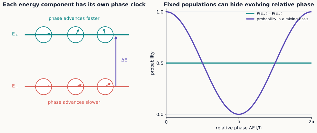
Figure 1:Energy-basis populations stay fixed while the phase clocks advance at rates set by their energies. Only the relative clock angle is observable, and a measurement in a mixing basis converts it into an oscillating probability.
Example 4.1: a two-level superposition
Suppose and
Removing the physically irrelevant common phase gives the equivalent representative
The energy probabilities remain one half at all times. But in a basis built from coherent sums of and , the corresponding probabilities oscillate with frequency . If these two energy states are chosen as the basis of a spin- system, the and bases are familiar examples of such mixing bases.
Only energy differences drive observable phase changes
For two energy components, the cross term in any measurement probability contains a phase of the form
This predicts an experimentally visible angular frequency , a useful fact to remember, since it also gives a quick dimensional check: energy divided by has units of inverse time, as an angular frequency should. A common phase built from, say, the average energy of two levels drops out of every isolated-system probability, exactly like the overall phase discussed in Section 4.1.
Example 4.2: evolution from a nondiagonal matrix
In the basis, consider
The energy eigenstates are and , with energies . Because the identity commutes with ,
Applied to , and suppressing the common phase,
Therefore
Notice what is happening here: the initial state was definite along , but the Hamiltonian was not diagonal in the basis. It is exactly this mismatch—the off-diagonal entries connecting and —that drives coherent transfer between the two outcomes over time.
4.3 Spin in a uniform magnetic field
We now specialize the general machinery above to the physical situation that will occupy the rest of this chapter: a spin in a magnetic field. A magnetic moment in a uniform field has Hamiltonian
the same energy expression introduced in Chapter 1, now promoted to an operator. For a spin- particle whose magnetic moment is proportional to its spin, write , where is the gyromagnetic ratio. For , this becomes
The sign of depends on the sign convention chosen for . Keeping track of that sign carefully, rather than dropping it, avoids silently reversing the direction of precession later on.
Because , its exponential can be evaluated directly from the power series, without any diagonalization step. Every even power of collapses back to , and every odd power collapses back to itself: , , and so on. Writing for brevity and separating the exponential’s power series into its even and odd terms,
using for even and for odd to pull out of every odd term. The two bracketed sums are exactly the ordinary Taylor series whose sum is and respectively: the same series reviewed above for , now split into its even and odd parts instead of read off directly. This gives
The identical argument applies to for any unit vector , since as well; this is exactly the fact reused in Section 4.5 for a field pointing in an arbitrary direction and in Section 4.10 for a general control pulse.
In the basis, where is already diagonal, this is simply
Concept check 4.2
A spin begins in in a uniform -directed field. Does it precess into ?
Answer
No. It is an energy eigenstate and gains only an overall phase. A state with a component transverse to the field has a Bloch vector that visibly precesses.
4.4 Larmor precession
The matrix above shows that a or state, being an eigenstate of , only picks up a phase and never changes. To see the field actually do something visible, we need a state with some component transverse to . Prepare and let it evolve in the -directed field. Then
After removing an overall phase, the relative phase between the two terms is , and Chapter 2 already showed exactly what a relative phase like this does to measurement probabilities in a different basis. The probabilities for a later measurement are
Meanwhile at every time : the -basis populations never change at all. Geometrically, the Bloch vector simply rotates around the axis at the Larmor angular frequency . This is the general pattern to remember: dynamics changes a relative phase, and it is the choice of final analyzer that converts an otherwise hidden phase into a measurable probability.
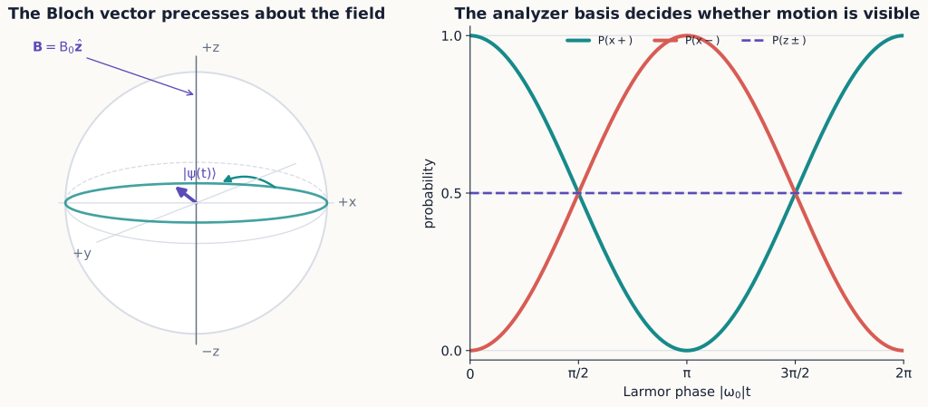
Figure 2:Larmor precession leaves the -basis populations unchanged but moves the Bloch vector around the equator. An analyzer reveals this motion as complementary oscillations in its two output probabilities.
Concept check 4.3
A spin in a -directed field always has . Must its state be constant in time?
Answer
No. Its relative phase may evolve even while its probabilities remain fixed. An or analyzer can reveal that phase evolution through changing counts. A single measurement basis does not provide complete state information.
This experiment is a two-state interferometer, in the same spirit as the recombination experiments of Chapters 1 and 2. Preparing creates two equal -basis amplitudes, the field gives them different phases as time passes, and the final analyzer recombines those amplitudes into an interference pattern. The observed oscillation is the spin-space analog of moving a phase plate through one arm of an ordinary path interferometer.
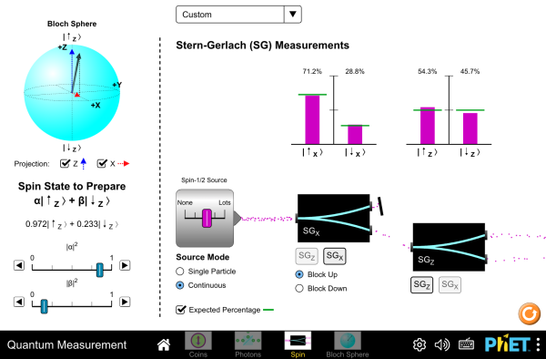
Figure 3:Prepare , switch on a -directed field, and watch the Bloch vector sweep around the equator at the Larmor frequency exactly as equation (25) predicts, while a live readout of confirms equation (26).
Interactive simulation: Quantum Measurement: Bloch Sphere
The classical system with the same equation of motion is a gyroscope: a torque perpendicular to an angular momentum does not tip it over but walks it around a cone at fixed polar angle, exactly as a transverse field walks the Bloch vector around the equator without changing .
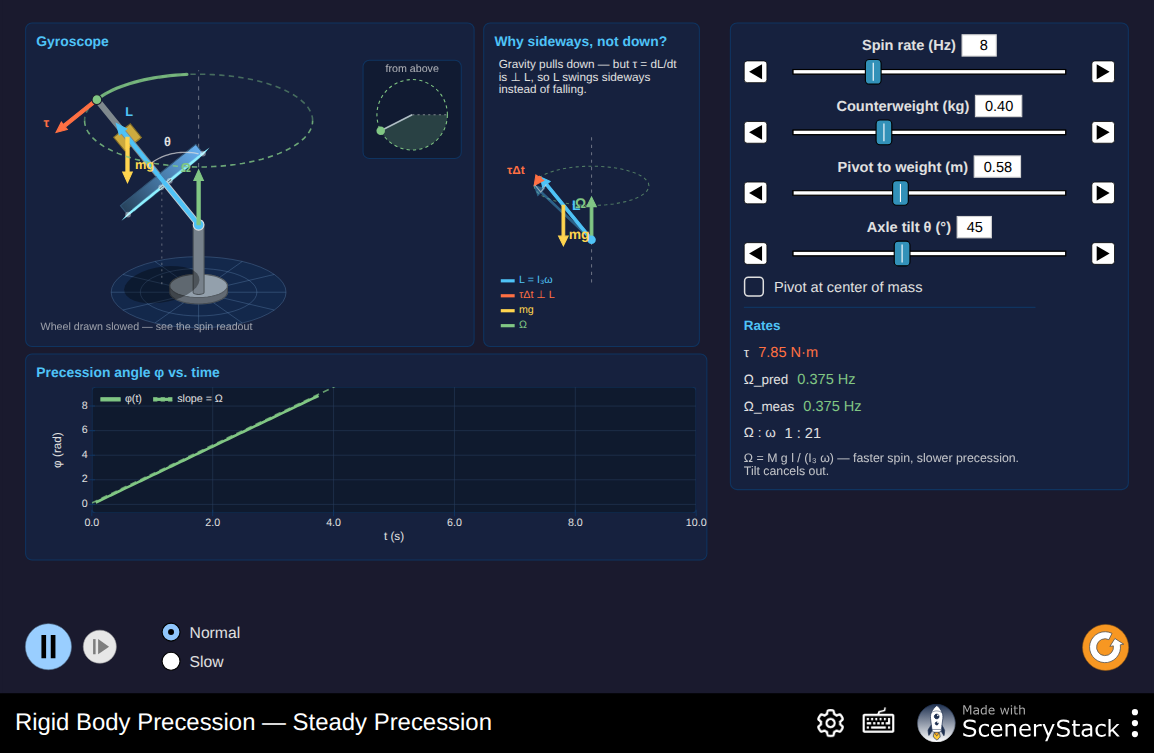
Figure 4:A spinning top under gravity, precessing steadily about the vertical. and stay fixed while and trace out a circle—the classical motion behind the Bloch vector’s rotation above, and behind the orbital-angular-momentum vector model of Chapter 9.
Interactive simulation: Precession
Example 4.3: a spin-flip time
Starting from , the first time at which an measurement gives with certainty satisfies . Thus
Be precise about what this is not: it is not a transition between the energy levels, since their populations remain fixed throughout. It is a rotation of the state relative to the measurement basis—the energy eigenstates are untouched; only the relative phase between them has advanced by .
Example 4.4: infer a field from counts
A state evolves for in a -directed field. A later measurement gives . Equation (26) implies
The smallest positive phase is , giving
Two ambiguities remain, and neither should be overlooked. The probability alone does not determine the sign of , since cannot distinguish clockwise from counterclockwise rotation. And because the cosine is periodic, this same data is also consistent with larger frequencies differing by whole cycles. Additional measurements at other times, or a analyzer sensitive to the direction of rotation, remove these ambiguities.
4.5 A field in an arbitrary direction
Everything so far assumed the field points along . For a constant field along an arbitrary unit vector ,
Since —the same identity used in Chapter 3—the same power-series trick used for generalizes immediately:
This operator rotates the Bloch vector around , and it also reveals why the exponent naturally involves a half-angle, echoing the half-angle rule from Chapter 1. A spatial rotation gives , and only a rotation returns the ket to exactly itself. That minus sign after is an overall phase for one isolated evolving path, so it has no effect by itself, but it becomes observable through interference with a second, unrotated path.
Three geometric cases deserve separate attention. If the initial Bloch vector is parallel to , the state is an energy eigenstate and gains only an overall phase, never changing direction. If it starts perpendicular to , it sweeps out a full circle around . At any intermediate angle, it traces a cone around , with its component along staying fixed throughout.
Example 4.5: rotation about 
Take the Hamiltonian and initial state . Equation (31) gives
The probability of a result is . At , the state has equal probabilities but a definite transverse direction; at , it is up to phase. Equal populations halfway through the rotation do not mean coherence has been lost, however: the state is still a perfectly definite pure state, just one pointing along a different axis.
4.6 Measurement interrupts unitary evolution
So far we have evolved a state continuously and only asked about measurement at the very end. Real experimental protocols often measure, select an outcome, and then let the resulting state evolve further, and it is important to know exactly how to handle that. Suppose the spin evolves until time , when is measured. Just before the measurement,
The outcome probabilities follow from projecting this state onto , exactly as in Chapter 3. If the result is , the state used for all subsequent evolution is itself, not the pre-measurement superposition:
Unitary evolution and ideal projective measurement are two genuinely distinct parts of the model, governed by different rules, and confusing them leads to a common mistake: continuing to evolve the pre-measurement superposition after a definite outcome has already been selected, as if the measurement had never happened.
Example 4.6: a complete prepare–evolve–measure protocol
A spin is prepared in , evolves in a -directed field for a time , and is measured along . Suppose the outcome is selected. The same field then acts for another time before a final measurement.
Just before the intermediate measurement, . Selecting prepares ; it does not leave the earlier phase-evolved ket in place, per the rule just stated. Starting fresh from , another quarter-period of evolution produces equal final probabilities. So the probability for either final result, conditional on having selected the branch, is . The probability for the complete route starting from the original preparation must also include the probability of the intermediate selection itself, giving overall.
4.7 Constants in the Hamiltonian
Adding a constant energy to every state changes the Hamiltonian to . Because commutes with anything, the corresponding evolution operator factors cleanly:
Every state acquires exactly the same overall phase from this shift, so isolated-system probabilities are completely unchanged. This confirms a pattern seen throughout the chapter: it is energy differences, not an arbitrary choice for the zero of energy, that control observable relative phases.
4.8 Optional mathematical extension: time-dependent Hamiltonians
Every result so far assumed a time-independent Hamiltonian, which is what let us write so simply. If instead changes with time, that simple exponential formula no longer applies, and the evolution operator must instead be defined through its own differential equation:
If the Hamiltonians at different times all commute with each other, the solution still takes a simple exponential form, just with an integral in place of a product:
But if for some pair of times, this shortcut fails, and the ordering of successive infinitesimal rotations genuinely matters; a time-ordered exponential or a piecewise product must be used instead. For example, a pulse about followed by a pulse about generally does not produce the same final state as the reversed sequence. This is the dynamical counterpart of the noncommuting analyzer questions from Chapter 3.
Example 4.7: a piecewise-constant Hamiltonian
Suppose a control system applies
Within each interval the Hamiltonian is constant. The complete evolution is therefore the ordered product
The earliest operation stands nearest the initial ket. Starting from , the first interval gives . Applying the rotation then gives
The displayed phase is overall, so the final Bloch direction is . If the two intervals are reversed, the pulse first changes only by an overall phase, after which the pulse leaves the Bloch vector at . The two schedules use the same Hamiltonians for the same durations but end in different physical states because the interval propagators do not commute. This piecewise construction is the practical finite-step version of time ordering.
4.9 Optional mathematical extension: motion of expectation values
The Schrödinger equation for the ket also implies a direct equation of motion for the expectation value of any observable, which is often a faster route to physical insight than tracking the full ket. For an operator with no explicit time dependence of its own,
Specializing to and using the spin commutators from Chapter 3, this becomes
Equation (42) has exactly the form of classical magnetic precession, even though each individual component measurement remains fully quantized, with only two discrete outcomes. It offers a useful bridge between two pictures developed so far: the geometric Bloch-sphere picture of Chapter 2, and the explicit matrix evolution of a ket developed in this chapter. The expectation vector traces out a smooth, classical-looking trajectory, even though the individual Stern–Gerlach outcomes behind it remain discrete.
4.10 Applications track: controlled rotations and pulse language
Laboratory control of a spin is usually described not in terms of a continuously running field, but in terms of discrete pulses—a field switched on for a controlled duration to produce a specific rotation. A constant control Hamiltonian applied for a chosen duration implements exactly such a rotation. Define
For applied for time , the rotation angle is . This control Hamiltonian is defined with the opposite sign from the field Hamiltonian of Sections 4.3–4.5; matching the two conventions, , recovers from equation (31). Two particular pulses come up often enough to deserve names: a pulse carries a Bloch vector to the opposite side of its rotation circle, while a pulse can turn a definite state into an equal-amplitude superposition. For example,
The factor may be dropped here because it multiplies the entire state; subsequent unitary operations cannot turn a truly global phase into a relative one. In multibranch calculations, however, a phase belonging to only one branch is not global and must be retained until the branches are recombined.
If an pulse acts first and a pulse second, the combined operator is
Read this expression from right to left: the earliest operation in time stands closest to the initial ket. Rotations about different axes generally do not commute, so reversing the order of these two matrices describes a genuinely different laboratory sequence, not merely a different way of writing the same one.
Example 4.8: pulse order on a prepared spin
Begin in . An -axis pulse produces
A subsequent -axis pulse changes this eigenstate only by an overall phase, since is already an eigenstate of the rotation axis. In the reverse order, the first pulse produces , which the pulse then changes only by an overall phase, for the same reason. The two final Bloch vectors, and , are clearly different states. This geometric shortcut reaches the same conclusion as direct matrix multiplication, with considerably less arithmetic.
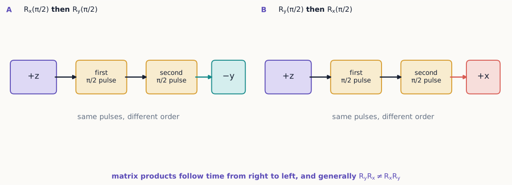
Figure 5:The same two control pulses lead to different final states when their order is reversed. The laboratory sequence runs left to right, while the corresponding operator product acts on the ket from right to left.
4.11 Applications track: Ramsey interference
We can now assemble everything in this chapter into one of the most important protocols in atomic physics: a Ramsey sequence, which is really an interferometer built entirely in a two-state space, using pulses instead of beam splitters. The protocol has five steps:
prepare ;
apply to create ;
allow free phase evolution for time ;
apply ; and
measure .
Represent the free evolution in step 3 by
where is the relative angular frequency in the chosen reference frame. Combining all five steps, the final state is
Projecting onto gives the observed fringes
It is worth naming what each step contributes: the first pulse creates two coherent amplitudes out of a single definite state, free evolution changes their relative phase by an amount set by and , and the second pulse recombines those two amplitudes so that the final measurement can read out the accumulated phase as a probability. This is precisely the coherent path logic first introduced in Chapter 2, now implemented with controlled rotations rather than physically separated paths.
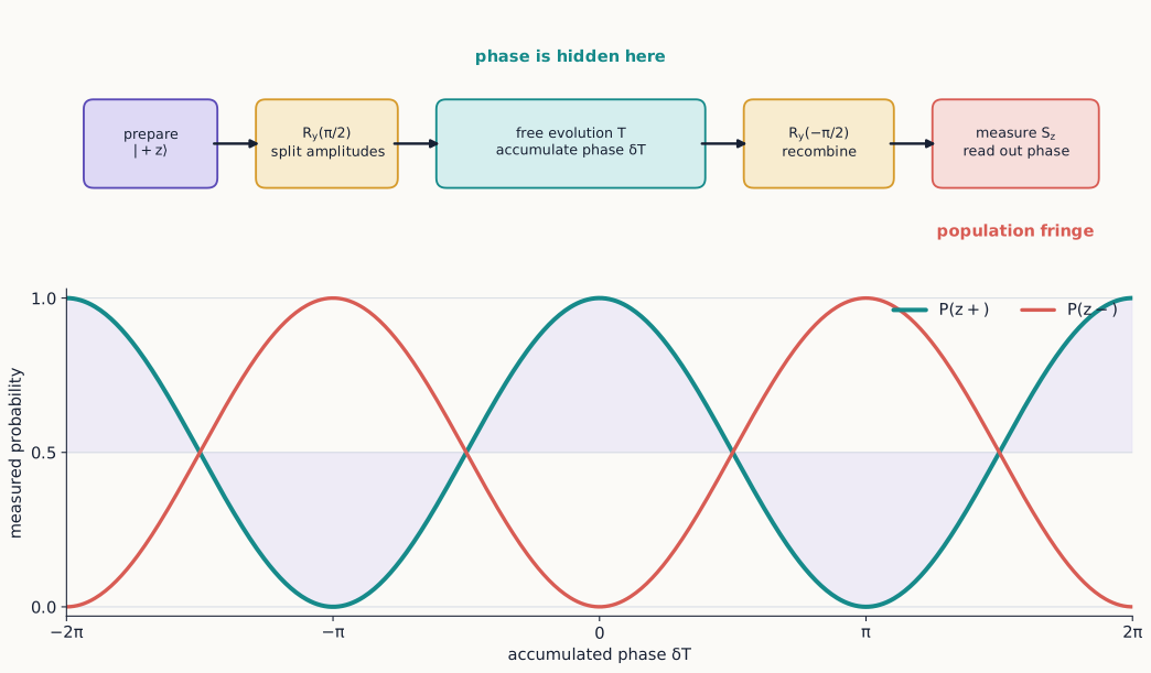
Figure 6:A Ramsey experiment is a two-state interferometer: the first pulse splits an amplitude, free evolution shifts the relative phase, and the second pulse recombines the alternatives. The final counts trace the accumulated phase as complementary fringes.
Example 4.9: the first fringe minimum
If , the first minimum occurs at :
Scanning at fixed detuning reveals these oscillations directly. Scanning the control frequency instead, at fixed , also produces fringes, now as a function of detuning rather than time. This sensitivity of a simple probability to a small phase is the operating principle behind atomic clocks and many modern quantum sensors.
If the accumulated phase varies unpredictably between different trials of the experiment, averaging over those trials reduces the fringe contrast. Each individual run may still be perfectly unitary; it is the pooled ensemble that becomes mixed, because its relative phase is no longer controlled from run to run. Density operators, introduced in Chapter 3, are exactly the tool needed to distinguish this loss of ensemble coherence from ordinary, coherent precession.
Concept check 4.4
Why not measure after the first Ramsey pulse to verify both alternatives?
Answer
That measurement would make the alternatives distinguishable and remove their coherence. If its outcomes were pooled, the second pulse would yield equal final probabilities rather than a full-contrast fringe.
Summary
The Hamiltonian generates deterministic, unitary evolution between measurements.
Energy eigenstates acquire only overall phases and are stationary.
Superpositions acquire changing relative phases set by energy differences.
A uniform magnetic field rotates a spin state; a field gradient can analyze it.
Larmor precession converts phase evolution into oscillating measurement probabilities.
Adding a constant to every energy changes only an unobservable overall phase.
A complete dynamics calculation specifies a preparation, an evolution operator, and a final measurement basis.
Time-dependent Hamiltonians require attention to the order of rotations when the Hamiltonians at different times do not commute.
Spin expectation values precess smoothly even though individual component measurements have only two discrete outcomes.
Controlled pulses implement rotations whose matrix order follows the laboratory sequence from right to left.
Ramsey sequences turn accumulated relative phase into measurable population fringes.
Exercises
Exercises 1–9 establish the core evolution and measurement workflow. Exercises 10–13 consolidate spin precession and interrupted evolution. Exercises 14–20 support the optional mathematical and applications tracks; a focused first assignment need not include all three groups.
Starting from equation (1), show directly that the norm of a state is constant when is Hermitian.
A two-level system has energies 0 and . Evolve the initial state and find the probability of returning to the initial state at time .
Derive equation (23) by separating the exponential power series into even and odd powers.
Derive equation (26) from equation (25) using inner products.
For the same evolving state, calculate and identify the direction of precession for positive under the conventions used here.
Find the earliest time at which a spin initially in becomes under a uniform field in the direction.
Prove that equation (31) is unitary.
An measurement is made halfway through a full Larmor period and its result is selected. Describe the state immediately before and after the measurement, then find one quarter-period later.
Show that adding to a Hamiltonian cannot affect the expectation value of any time-independent observable in an isolated system.
For the Hamiltonian in Example 4.2, calculate for an initial state. At what earliest time is the state up to overall phase?
A state precesses in a -directed field. Find both and , and explain how their relative timing reveals the sign of .
Derive the result of Example 4.5 by expanding in the energy basis , evolving the two components, and transforming back.
Work through every branch of Example 4.6 rather than selecting only . Show that pooling the intermediate outcomes gives final statistics different from a protocol with no intermediate measurement.
A Hamiltonian equals for a duration and then for the same duration. Write the total evolution operator in the correct order. Repeat for the reversed pulse sequence and show that the results differ unless takes a special value.
Derive equation (41) from the Schrödinger equation and its Hermitian conjugate.
Use equation (42) to identify a conserved component of in a constant magnetic field and connect it to energy conservation.
Verify both pulse actions following equation (43) using explicit Pauli matrices.
Calculate both pulse orders in Example 4.8 by matrix multiplication.
Insert an unread measurement after the first Ramsey pulse and use density operators to show that both final outcomes have probability .
Selected exercise guidance
Use these answers only after making a complete attempt.
Exercise 2
The return amplitude is , so the return probability is .
Exercise 5
For positive under the chapter’s sign convention, the Bloch vector is and
It initially moves from toward .
Exercise 6
, so the earliest certain flip occurs at .
Exercise 19
At , the probabilities are respectively ; the probabilities are the complements.