Stern–Gerlach experiments
Learning objectives
After this chapter, you should be able to:
describe preparation, analysis, and detection in a Stern–Gerlach experiment;
predict qualitative outcomes of sequential analyzers;
calculate route probabilities and expected counts for analyzers at arbitrary relative angles;
distinguish an incoherent mixture from a coherent quantum state;
infer three empirical rules that a quantum model must reproduce;
explain why spin is not adequately modeled as a tiny classical arrow;
distinguish ideal probabilities from finite-sample frequencies; and
design analyzer sequences that test competing physical explanations.
The final two objectives are developed in optional laboratory and inquiry extensions after the chapter’s core conceptual sequence.
1.1 An experiment before a formalism
Quantum mechanics is easiest to trust when it grows out of a real experiment, rather than being handed to you as a list of abstract postulates. So this book begins with one of the simplest experiments in physics: the one performed by Otto Stern and Walther Gerlach in 1922. Their question was simple. Does an atom’s magnetism point in only a few special directions, or can it point anywhere at all? The answer they found was strange enough to force physicists to rethink what it even means for a particle to have a direction.
Picture the apparatus in three stages. First, an oven heats a sample of silver until atoms boil off as a vapor. Second, that vapor escapes through a narrow opening, and a pair of slits downstream accepts only atoms traveling within a narrow range of directions; what emerges is a collimated beam. Collimation does not, by itself, select one exact speed: an oven beam retains a thermal spread of speeds unless a separate velocity selector is added. In the idealized diagrams below we suppress both spreads so that the spin-dependent splitting is easy to see. Third, the beam passes between the shaped poles of a magnet and then strikes a glass screen, where each atom leaves a visible mark.
One feature of the magnet matters more than any other: its poles are shaped so that the field is much stronger near one pole than the other. Without this asymmetry the experiment would show nothing interesting, as the next few paragraphs will make clear.
To see why the asymmetry matters, picture each atom as a tiny bar magnet, described by a magnetic moment vector —the same quantity that tells a compass needle which way to twist. Just like a compass needle, the atom’s energy depends on how is oriented relative to the external field : lined up with the field is low energy, opposed to the field is high energy, and every angle in between interpolates smoothly. In symbols,
A uniform field, however, cannot push the atom anywhere—it can only twist it. The force pulling one “pole” of the tiny magnet forward is exactly canceled by the force pushing the other pole backward, so the atom feels a torque but no net force. A push appears only when the field itself is stronger on one side of the atom than the other, that is, only when the field has a gradient. For a gradient along the direction, the net force on the atom works out to
Equation (2) is the whole operating principle of the device. It says that each atom is pushed by an amount proportional to , the component of its magnetic moment along the gradient direction. A larger means a larger deflection; a reversed means deflection the other way. In short, the magnet turns an otherwise invisible internal property of the atom—its magnetic orientation—into something we can see directly: a spot’s position on the screen.
Now we can ask what classical physics predicts for the result. Nothing in classical physics picks out a preferred direction for , so the atoms emerging from the oven should have their magnetic moments pointing every which way. That means should take every value between and , depending on each atom’s orientation angle . Combined with equation (2), this predicts a continuous smear of deflections on the screen. For fixed-magnitude moments pointing isotropically, is uniformly distributed, so the idealized classical pattern is an approximately uniform band between the two extreme deflections. Thermal speeds, finite slits, and detector resolution can broaden or reshape that band, but they do not turn it into two discrete spots.
That is not what Stern and Gerlach saw. Instead of the predicted continuous band, their deposited silver pattern separated into two traces. In the ideal two-outcome model used throughout this chapter, we represent those traces as two spots labeled and .
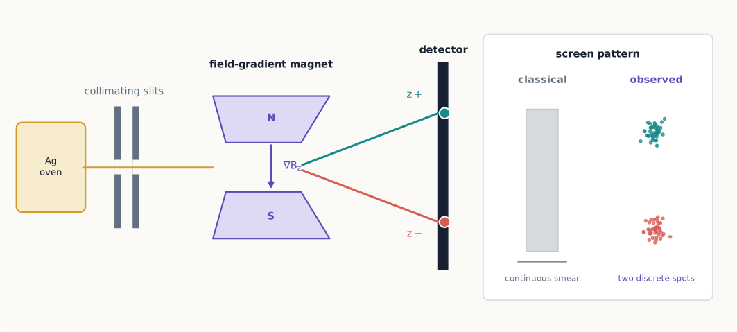
Figure 1:The Stern–Gerlach apparatus converts the spin component along the field gradient into a visible deflection. The decisive observation is not merely a deflected beam, but two discrete spots in place of the classical smear.
The two-spot pattern tells us something remarkable: the component of the atom’s magnetic moment that couples to the apparatus takes two discrete values rather than a continuum. Historically, Stern and Gerlach observed this space quantization before electron spin had been identified. In the modern description, a ground-state silver atom has closed inner shells and one unpaired outer electron with zero orbital angular momentum, so its relevant two-valued angular momentum is spin. No matter which axis we build the magnet along, an analyzer of this effective spin- system produces only two outcomes—never a value in between. The measured component can only be
This restriction—only two outcomes, no matter how the analyzer is oriented—is the first genuinely quantum fact in this book. Everything that follows is an attempt to build a mathematical theory around it.
From now on we abbreviate an analyzer oriented along as . Something useful happens if we place a physical block in front of one of its two exits. Say we block the exit and let only the beam through. Every atom that makes it past the block is now guaranteed to have been recorded as —so the same device that just measured spin has become a device that prepares it. This dual role, one physical apparatus used first as a measurement and then as a preparation, will come up again and again in this chapter, so it is worth fixing firmly in mind now.
Reading the experiment from left to right
To talk about these experiments precisely, it helps to separate every one of them into three stages:
A preparation specifies how the incoming ensemble was made. A source by itself may be unpolarized; a source followed by a filter prepares a selected spin state.
A transformation changes the state without yet recording a spin result. Examples include a uniform magnetic field or a coherent path recombiner.
A measurement ends in macroscopically distinguishable records, such as counts at the two exits of an analyzer.
This vocabulary heads off a common confusion. The symbol gets used for three different things: an outcome recorded at a detector, the physical exit path leading to that detector, and the state that gets prepared when we select that path. Context usually makes clear which meaning is intended, but keep in mind that these are three related, not identical, ideas.
In the laboratory, what we actually observe are raw counts: some atoms land in the spot, some in the spot. If and are the numbers of atoms detected at the two exits, the measured relative frequencies are
Quantum theory predicts the probabilities that these frequencies approach after many repetitions of the same experiment. It does not, in general, predict which exit any one particular atom will take.
1.2 Repeatability
Here is the simplest possible follow-up experiment: put a second analyzer right after the first one, oriented along the same axis, and keep only the atoms that came out of the first analyzer’s exit. What happens at the second analyzer?
The answer is unambiguous: every atom that enters the second analyzer leaves through its exit. None comes out .
This tells us that the first analyzer did more than sort atoms into two piles. Selecting the output prepared something new: a beam in which every atom is now definite for a repeated measurement, meaning that measuring it again along can no longer produce a surprise.
Repeatability also gives us an operational definition of the label , which will be introduced formally in Chapter 2: it means the preparation that produces with certainty when immediately analyzed along . We do not need to imagine what the atom is “really doing” between devices in order to define the state reproducibly.
Example 1.1: counting atoms
A source sends atoms into . The source has no preferred orientation, so half emerge from each exit on average. The exit is blocked, and the beam enters a second .
About atoms reach the second analyzer, and all leave its exit. Statistical fluctuations affect the first split, but an ideal repeat measurement does not create a second 50–50 split.
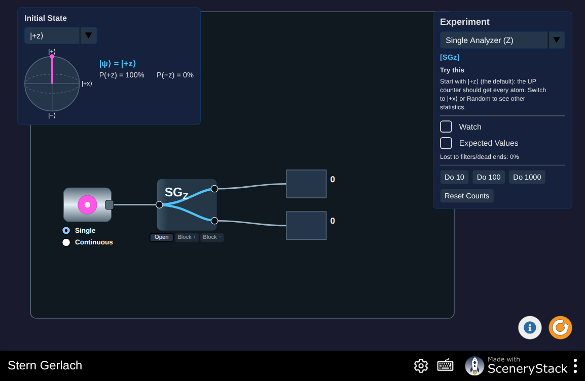
Figure 2:Assemble your own chain of ovens, analyzers, and counters, fire spin- or spin-1 atoms through it, and watch Monte Carlo counts accumulate next to the analytic prediction. Rebuild the repeated-analyzer setup from Example 1.1 before reading on, then try chaining analyzers at other angles.
Interactive simulation: Stern Gerlach
1.3 Incompatible questions
Repeating a measurement along the same axis gave a simple, if important, result: nothing changes. The next natural question is what happens if we measure along a different axis instead. Prepare a beam as before, but this time send it into , an analyzer whose field gradient points along rather than . The output divides equally:
So a preparation is not definite for : knowing that an atom is tells us nothing about which way it will go in . Here is the more surprising part. Keep only the output of that measurement, and send those atoms into a third analyzer, this one measuring again. If the atom really still had a definite value all along, we should recover with certainty, exactly as in Section 1.2. Instead, both outcomes now occur with equal probability, as if the intervening measurement had erased what we thought we already knew:
This is the key point: measuring changed what we could predict about , even though nothing directly measured in between. It is tempting to imagine that the atom secretly carried permanent values for both and , and that each analyzer simply reads the relevant value without changing anything else. The experiment rules out that specific, noninvasive fixed-label model: if the analyzer merely revealed an unchanged label, the final measurement should still return with certainty—but it does not. The sequence does not, by itself, rule out every possible hidden-variable account; a more elaborate model could allow the apparatus to alter hidden variables contextually. Bell’s test in Chapter 5 will impose additional locality assumptions and reach a stronger conclusion.
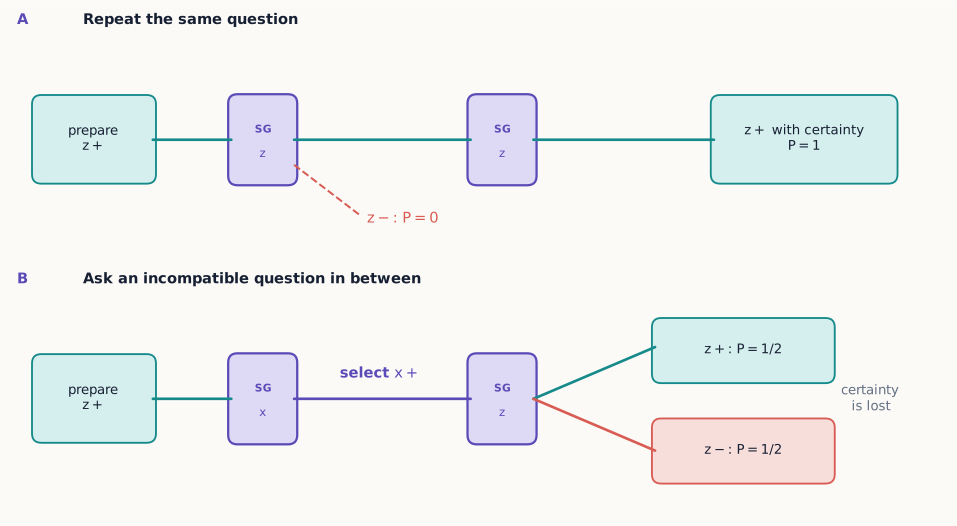
Figure 3:Aligned analyzers repeat a definite result, whereas an intervening analyzer along an incompatible axis replaces that certainty with a new preparation. The diagrams are read from left to right, just like the laboratory sequence.
Concept check 1.1
A beam enters . The exit is blocked, and the transmitted beam enters another . What fraction of the original beam reaches the final detector?
Answer
One half. The first measurement transmits half the atoms into . Repeating the measurement then returns with certainty.
What “disturbance” does and does not explain
One might instead say that the middle analyzer simply adds uncontrolled mechanical noise. Repeatability shows why that description is inadequate: if the device only randomized everything, its own result would not be reliable on repetition. Yet an selection is perfectly repeatable. The analyzer performs a reproducible transformation—it replaces a preparation definite for with one definite for —even though the later result becomes uncertain. This does not prove that no underlying disturbance occurs; it shows that “mere random jostling” lacks the structure needed to explain the observations.
Order matters here in a way that has no classical analog. Compare
with
In the first sequence, repeating the measurement changes nothing, so the final analyzer still sees a 50–50 split, exactly as it would from a fresh beam. In the second sequence, the intervening selection changes the outcome seen by the final analyzer, turning certainty into a 50–50 split. Chapter 3 will express this order dependence precisely, as a statement about products of noncommuting matrices.
Analyzers at a general angle
So far we have only compared axes at and . What happens at angles in between? Nothing stops us from building an analyzer tilted at any angle relative to the preparation axis, and it seems reasonable to guess that the probability of recovering the original outcome should fall off smoothly as the analyzer tilts away from the preparation axis. If spin behaved like an ordinary arrow, we might guess that this probability varies as , matching the projection of one vector onto another. Experiment gives a different, and at first surprising, answer. For a beam prepared spin-up along and analyzed along , separated by angle ,
Notice the half-angle, , rather than itself. This is not a typo or a minor detail—it is an early hint that spin does not transform like an ordinary arrow in space. As Chapter 4 will show, a representative spinor acquires an overall minus sign under a rotation and returns to the identical ket only after . The minus sign does not change the physical state of an isolated spin, because overall phase is unobservable; it becomes detectable only relative to another coherent amplitude. The half-angle in equation (9) is an early fingerprint of this spinor transformation law.
It is worth checking that this formula reproduces everything found so far. At (aligned analyzers), : certainty of recovering the same outcome, matching Section 1.2. At (oppositely aligned analyzers), : certainty of the opposite outcome. At (perpendicular analyzers, like versus ), : an equal split, matching Section 1.3. Equation (9) is therefore not a separate new rule; it is the general law that contains every case already found as a special case. For now we treat it as an empirical summary of the data. Chapter 2 will derive it from the mathematics of state vectors.
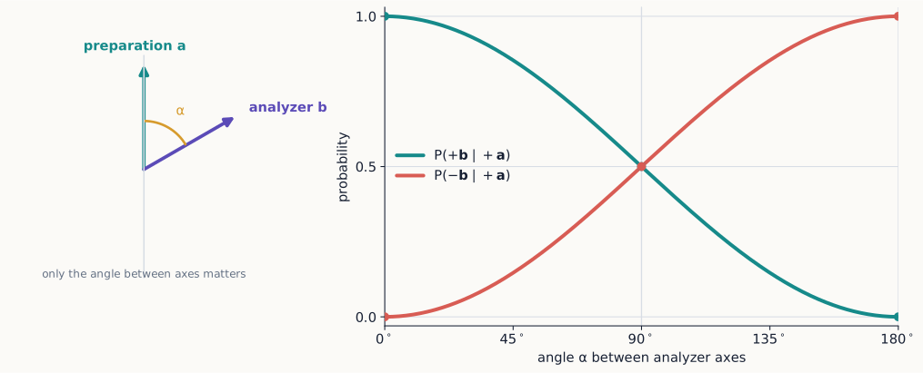
Figure 4:The half-angle rule smoothly joins repeatability at , equal splitting at , and certain reversal at . At every angle the two exclusive probabilities add to one.
Example 1.2: three analyzer directions
A beam passes through an analyzer whose axis is from , and only the output is retained. That beam is then measured along . This means applying equation (9) twice in a row, using the selected output of the first analyzer as the input to the second.
At the middle analyzer, equation (9) applies with , so the half-angle appearing in the formula is :
The selected middle output is a new preparation. Since the angle back to is again ,
Thus of the original atoms reach the final detector and reach the final detector; the remaining quarter was blocked at the middle analyzer. Conditional probabilities must be multiplied along a selected path.
Concept check 1.2
A beam is analyzed along an axis only from . One student predicts exactly because the axes are nearly aligned; another predicts a 50–50 split because the axes are different. What does the experiment predict?
Answer
Neither. The probability of is , while the probability of is about 0.0076. Quantum outcomes are discrete, but their probabilities vary continuously with analyzer orientation.
1.4 Recombining alternatives
Every experiment so far has ended with a measurement: an atom lands in one detector or another, and that is the end of the story. What happens if, instead of recording which path an atom took, we let two paths recombine before anything is measured?
Imagine a carefully built device that splits a beam into two separate paths, one associated with and one with , and then brings the two paths back together—coherently, without ever revealing which path a given atom traveled. Remarkably, the recombined beam turns out to be back in the original state, exactly as if the device had never touched it. But if we block either path, so that only atoms from the other path get through, the later statistics change completely.
This kills a natural but wrong guess: that the two paths behave like two ordinary, independent sub-beams, so that whatever happens to the recombined beam should just be the sum of what happens along each path separately. Quantum theory instead assigns a complex number—a probability amplitude—to each indistinguishable alternative. When alternatives are indistinguishable, we add the amplitudes first, and only afterward take the squared magnitude to get a probability.
This distinction will later become the difference between a coherent superposition and an incoherent mixture.
The word coherently carries real experimental content. The apparatus must preserve a stable relation between the phases accumulated on the two paths. If vibrations, stray fields, or a path detector randomize that relation, the interference washes out even when nobody reads the detector. What matters is whether a durable physical record could distinguish the alternatives, not whether a person happens to look.
One can summarize the alternatives with two limiting arrangements:
Both paths open and recombined: add the two complex amplitudes, including their relative phase, and then square the magnitude.
Paths detected separately or phase-randomized: square the magnitudes for the alternatives separately and then add the probabilities.
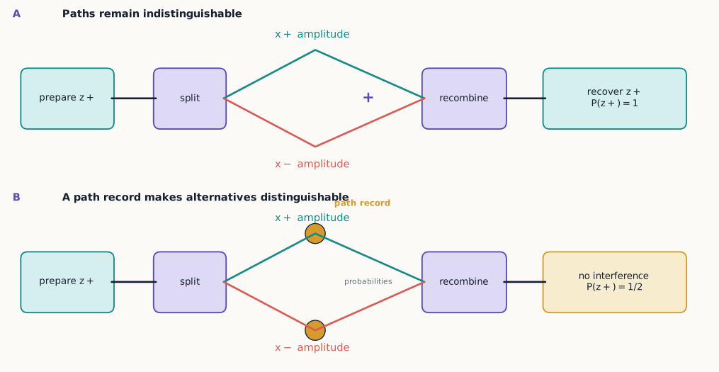
Figure 5:Recombination restores the original state only while the two alternatives remain coherent. A durable path record changes the calculation from adding amplitudes to adding probabilities, even if nobody reads the record.
This is why “half the atoms went through each arm” is not a complete description of the coherent experiment. The path amplitudes can cancel at one output and reinforce at another, even though each open arm alone sends atoms to both outputs.
Concept check 1.3
Why is a 50–50 collection of separately prepared and atoms not automatically equivalent to a coherent recombination of the two paths?
Answer
The collection records mutually exclusive preparations and is an incoherent mixture. A coherent recombination preserves the relative phase between the two amplitudes, so later probabilities can contain interference terms.
1.5 A minimal model
We now have three empirical rules—repeatability, incompatibility, and interference—plus the half-angle probability law. Before building a full mathematical theory, it helps to state in plain language exactly what that theory needs to accomplish:
A preparation is represented by a state.
A measurement has a discrete set of possible results.
A state assigns an amplitude, not directly a probability, to each result.
Measurement both produces a result and prepares a corresponding output state.
Different analyzer orientations represent different, sometimes incompatible, physical questions.
For spin , two independent states suffice to describe every possible pure spin state. We will represent them by vectors in a two-dimensional complex vector space. The word “two-dimensional” refers to state space, not ordinary physical space.
If “complex vector space” does not yet mean much to you, that is completely expected at this point—nothing so far has required it. Chapter 2 builds this idea from the ground up, starting with a review of ordinary arrows in the plane and of complex-number arithmetic itself, before ever writing down a spin state. The two-outcome rule, the incompatibility of and , and the interference rule found above are the experimental reasons that vector space is the right tool; the vocabulary comes second.
From laboratory rules to mathematical demands
Let’s translate the experimental facts directly into mathematical requirements. Whatever structure we build, it needs:
two mutually exclusive outcomes for each analyzer direction;
a way to represent a preparation that is certain for one outcome;
continuous families of other preparations, because the analyzer direction varies continuously;
a rule that produces normalized probabilities;
an update rule after an outcome is selected; and
phase information capable of describing coherent recombination.
An ordinary list of two probabilities, say , cannot do this job: it records the weight of each alternative but throws away the phase that controls interference. A pair of complex numbers can do both at once, since a complex number naturally carries both a magnitude and a phase. This is exactly why Chapter 2 introduces state vectors with complex-number coefficients—called kets—before ever writing down a wavefunction.
1.6 What spin is—and is not
The name “spin” invites a picture: a tiny sphere spinning on its axis, like a planet. That picture is a useful crutch for the imagination, but it is not literally correct, and taking it too literally leads to wrong predictions. Spin does carry angular momentum, and often a magnetic moment, which is exactly why it interacts with the field in a Stern–Gerlach apparatus in the first place. But a rigid, rotating sphere would have a magnetic-moment component that varies continuously as its axis tilts—precisely the smooth spread that classical physics predicted and that the apparatus did not show. The name “spin” is a historical label; it is the experiments, not the name, that tell us what spin actually is.
There is a second way the arrow picture fails, beyond just the two discrete outcomes. A classical arrow pointing at a known angle to the analyzer would have a projected component proportional to , and that component would vary continuously as varies. Real spin does not do this: the outcome is always , and the angle only controls how often each outcome occurs, through equation (9).
One more warning about pictures. Chapter 2 introduces the Bloch sphere, which looks like a sphere covered in little arrows. Resist the urge to picture each arrow as a literal miniature compass needle sitting inside the particle. Each arrow is shorthand for an entire preparation recipe and the statistics it produces—not a claim that the particle contains a tiny spinning pointer.
1.7 A systematic way to predict analyzer chains
Until the vector formalism is available, a short operational recipe is enough for ideal sequential measurements:
Identify the state entering the first analyzer. If the source is unpolarized, the first analyzer produces equal counts.
At each analyzer, measure the angle from the most recently selected preparation axis, not necessarily from the original axis.
Use equation (9) for each branch.
Multiply conditional probabilities along one branch; add probabilities only when mutually exclusive detected branches are pooled.
If paths are recombined coherently, stop using this probability-tree recipe. Amplitudes and their phases are then required.
Example 1.3: keep all branches straight
An unpolarized source sends atoms into . The exit is selected, then the exit of an analyzer is selected, and finally both exits of are counted.
The expected bookkeeping is
The final counts are not and zero. The state entering the last analyzer is , not the earlier preparation. Writing the state beneath each segment of an apparatus sketch is a simple way to avoid this mistake.
1.8 Optional laboratory extension: from probabilities to data
The conceptual route to the state-vector formalism is complete at this point. This optional section connects ideal probabilities to the fluctuations and systematic effects encountered in laboratory data.
Equations such as (9) predict probabilities, whereas a real experiment produces integer counts. The link between the two is statistical.
If the preparation and analyzer are held fixed and independent atoms are recorded, the number at the positive exit fluctuates around , where
For ideal independent trials, the count follows a binomial distribution. Its standard deviation is
and the measured frequency has standard deviation
The dependence matters. Recording four times as many atoms reduces the typical frequency fluctuation by only a factor of two. Quantum theory does not predict that every batch divides in exactly the theoretical ratio; it predicts the distribution of results from which those batches are drawn.
Example 1.4: is a split consistent with the angle rule?
A source is analyzed along an axis from . Among detected atoms, leave the positive exit. The ideal prediction is , so the expected count and its standard deviation are
The observed count is 15 below the mean, about 1.1 standard deviations. Such a difference is ordinary statistical variation, not persuasive evidence against the angle rule. By contrast, a persistent discrepancy that grows in statistical significance as more data are collected suggests imperfect preparation, a misaligned analyzer, unequal detector efficiencies, or a failure of the model.
Concept check 1.4
A run with 100 atoms gives 54 counts at and 46 at . Has the expected 50–50 split failed?
Answer
No. For and , the expected standard deviation of the positive count is . A count of 54 is less than one standard deviation above the mean of 50 and is entirely typical.
Estimating an unknown analyzer angle
The same experiment can be used in reverse. For a known input and an analyzer known to lie between 0 and from , the observed positive frequency estimates the angle:
If of a large sample exits through , then . Counts can therefore characterize an apparatus as well as test a prepared state. In later chapters, this reversal of viewpoint becomes quantum-state tomography: known analyzers are used to infer an unknown preparation.
1.9 Optional inquiry extension: separating competing explanations
This optional section turns the chapter’s observations into a model-testing strategy: choose arrangements for which plausible explanations make different predictions.
A useful experiment does more than exhibit an effect; it distinguishes between models that would otherwise make the same prediction. A single analyzer, on its own, cannot distinguish a genuine quantum state from a classical population of atoms carrying fixed labels—both would give the same repeatable result. Sequential analyzers are powerful precisely because they force competing stories to disagree.
Consider three hypotheses for a beam selected from the exit:
Fixed-label hypothesis: every atom carries permanent values for all analyzer directions, and an analyzer only reads the relevant value.
Classical-arrow hypothesis: every atom carries an ordinary magnetic arrow, and the analyzer reports its component along the chosen axis.
Quantum preparation hypothesis: selecting an outcome prepares a state definite for that analyzer, while other components generally remain indefinite.
The sequence is compatible with the first and third hypotheses, so repeatability alone does not decide between them. The sequence , however, restores a 50–50 distribution. That result conflicts with permanent, merely revealed labels. The fact that every analyzer still has only two exits conflicts with a classical arrow whose projected component can vary continuously. Coherent recombination then adds a third test: interference depends on a controllable relative phase that neither classical population model retains.
This pattern is a general method for reasoning in quantum mechanics:
list the preparations and recorded outcomes without adding an unseen story;
derive a quantitative prediction from each candidate model;
choose a sequence for which those predictions differ; and
repeat enough trials to separate systematic disagreement from count noise.
Example 1.5: measurement or mere beam splitting?
An ideal device separates a input into and paths. Compare three arrangements.
With both paths coherently recombined, a final analyzer returns with certainty.
With the path blocked, the final analyzer gives and equally.
With a path marker present but both beams physically redirected toward the output, the final analyzer again gives the incoherent 50–50 statistics if the marker records perfectly distinguishable alternatives.
The last comparison shows why spatial overlap alone is not sufficient for interference. The relevant condition is whether the alternatives remain coherent—whether any physical degree of freedom carries usable which-path information. Chapter 2 will represent this distinction by retaining or discarding the cross terms between amplitudes.
Concept check 1.5
Why can the sequence test more than the sequence ?
Answer
Both a fixed-label model and quantum theory can imitate immediate repeatability. They differ after an incompatible intermediate measurement: quantum theory predicts that selecting prepares a new state and makes the final result 50–50, whereas a device that merely reads a permanent label should not erase it.
Summary
A Stern–Gerlach analyzer correlates a spin component with one of two paths.
Filtering an output prepares a repeatable state for that component.
Orthogonal spin components are incompatible: preparing one makes another uncertain.
Indistinguishable alternatives interfere through complex amplitudes.
A spin- state requires a two-dimensional complex state space.
Analyzer chains are sequences of conditional preparations and measurements; the most recent selected outcome determines the state entering the next device.
Finite data fluctuate around theoretical probabilities with a characteristic scale proportional to .
Sequential and coherent-recombination experiments are valuable because they force classical and quantum explanations to make different predictions.
Exercises
Exercises 1–6 rehearse the core analyzer logic, 7–11 consolidate angle rules and coherent alternatives, and 12–16 extend the chapter into data analysis and experimental design. Complete the first group before choosing from the later two.
An unpolarized beam of atoms passes through ; the output then passes through . Estimate the counts in the two final outputs.
Predict the possible final outcomes and their probabilities for .
Insert a second after the selection in Exercise 2. Explain why its result differs qualitatively from the final result.
A student says, “The first analyzer tells us which atoms were already pointing up.” Identify two observations in this chapter that this classical explanation fails to capture.
Explain operationally what must be changed to turn a spin analyzer into a state-preparation apparatus.
Design a sequence of ideal analyzers that begins with and has a final detection probability of . Give at least two sequences and explain them.
A beam is sent to an analyzer tilted from . Find both output probabilities using equation (9).
An unpolarized beam of atoms passes through three analyzers. The selected outputs are first and then , where is from . Both outputs of the final analyzer are recorded. Predict all final counts and account for atoms blocked earlier.
Draw probability trees for and . If the two selected beams are later pooled incoherently, what are the final probabilities?
A two-path apparatus gives deterministic when both paths are open and recombined. With either path blocked, the final analyzer gives both results. Explain why adding the two single-path probability distributions cannot reproduce the both-open result.
Classify each element as preparation, transformation, or measurement: an oven source, a filter, a uniform magnetic field, an unobserved path marker, a coherent recombiner, and a two-channel detector. Some elements may play more than one role; explain your choices operationally.
A beam is analyzed from its preparation axis. In a run of atoms, estimate the mean and standard deviation of the count. Is a count of surprising on this scale?
A large sample prepared in gives at an analyzer whose axis is known to lie between and from . Estimate the angle.
Derive equation (15) from equation (14). Explain why the absolute uncertainty in a count grows with while the uncertainty in a relative frequency shrinks.
Design a three-configuration experiment that distinguishes coherent recombination, an incoherent mixture of the two paths, and accidental blocking of one path. State the qualitative final statistics expected in each configuration.
A source drifts so that its intensity falls by during a run. Explain why raw output counts could then give a misleading comparison between two analyzer settings. Propose a frequency or normalization that reduces the problem.
Selected exercise guidance
Use these answers only after making a complete attempt.
Exercise 2
The selection occurs with probability . Conditional on that selection, the final and probabilities are each , so each complete detected route contains of the original beam.
Exercise 7
and .
Exercise 12
The mean is and the standard deviation is . A count of is 1.6 standard deviations above the mean, so it is not especially surprising.