Abstract
In this chapter, we explore the fascinating world of particle physics and the Standard Model of Particle Physics. We discuss the constraints of the Schrödinger equation and the necessity of quantum field theory, introducing key concepts like antimatter, vacuum fluctuations, and Feynman diagrams. The chapter details the fundamental particles and forces in the Standard Model and highlights unresolved questions, such as dark matter, dark energy, and the integration of gravity. Additionally, we examine the role of virtual particles and the impact of vacuum fluctuations on our understanding of particle interactions. We aim to provide a comprehensive overview of the current state of particle physics and the exciting challenges that lie ahead.
Keywords: Quantum field theory, Standard model of particle physics, Quantum electrodynamics, Quantum chromodynamics, Antimatter, Particle physics, Vacuum fluctuations, Feynman diagrams, Beyond the standard model
Learning Goals
By the end of this chapter, you should be able to understand:
that quantum mechanics does a great job of describing the world of the super small, but it is not perfect.
that the Standard Model of Particle Physics is a conceptual model of the world of the super small; the mathematical framework for it is called Quantum Field Theory.
that the Standard Model of Particle Physics is not complete. There are problems with it, but we aren’t entirely sure how to make a more complete model. There are lots of ideas, but so far, no one has been able to experimentally confirm a better model.
11.1 Problems with Quantum Mechanics
We spent a lot of this book conceptually thinking about atoms. Many of the conceptual ideas come from quantum mechanics, which is mathematically described by the Schrödinger equation. Whenever you work with a model, it is important to know the limitations of your model. For example, you can’t use classical physics, like Newton’s second law, to describe the world of the super small. For things that are moving very fast,[1] we need Einstein’s theory of special relativity. The goal of fundamental science is to develop a model that accurately describes nature. Since we now have a good conceptual background on the world of the super small, let’s discuss the limitations of the quantum mechanical model.
Things moving fast: The Schrödinger equation is only for slow-moving-particles. However, physicists have incorporated the ideas and mathematical models of special relativity into the Schrödinger equation. But none of these did a complete job. If you are interested in this topic, you should search the internet for “the Dirac equation” and “Klein–Gordon equation.” Just a heads-up, the Wikipedia pages for these two equations are extremely mathematical. For completeness, folks also use something called perturbation theory that helps approximate the effects of fast-moving particles. It can do a really good job, but, in the end, perturbation theory is just an approximation.
Radioactive decay: The mathematical model behind quantum mechanics, the Schrödinger equation, conserves particle number.[2] This will be one of the first things you prove if you take a quantum mechanics class.[3] Particle conservation means if a particle exists at one point in time, it has always existed and will always exist. We know this is not true. We create and destroy particles all the time! This is the whole purpose of a particle accelerator. In addition, we already talked about radioactive decay. For example, during decay, a neutron stops existing and a proton, electron, and anti-electron neutrino come into existence. That means we went from 1 neutron to 0 neutrons. Particle number is definitely not conserved.
Excited state decay: An atom that has an electron in an excited state will decay to a lower energy state and emit a photon. This process is random and mathematically modeled by an exponential decay (this was talked about back in Chap. 3. Atoms at Rest if you need a refresher). However, to get an atom to decay, it needs to be acted upon from the outside. Think about how we need force (or torque) to change an object’s momentum (or angular momentum). But an excited state atom seems to decay all by itself with no external interactions.
Quarks: Physicists discovered that a proton is composed of three particles known as quarks. While we will talk more about quarks in Sect. 11.5 The Standard Model of Particle Physics, the really important thing here is that the mass of the three individual quarks is only about 1% of the mass of the proton. Think about that for a minute. Imagine I hand you 3 steel balls. You weigh each one individually and determine two of the balls have a mass of 2.2 grams and one of the balls has a mass of 4.7 grams. Now you put all 3 steel balls on the scale. A logical guess would say the total mass should be . Instead, you find that the mass is 938 grams. Replace grams with a much smaller unit for mass and you have what actually happens …
The speed of causality: Imagine you had two charged particles that are separated by a few meters. Next you nudge one of the charged particles. According to the Schrödinger equation (and also classical electromagnetic theory), the other particle reacts instantaneously. You could repeat this experiment with one of the charged particles on earth and the other on Mars and get the same result. The two charged particles feel a force from the other charged particle and if you move one particle, the other will instantaneously feel a force that pushes or pulls on it. This violates special relativity. Special relativity says the fastest anything can move, including information about where a particle is located, is 299,792,458 m/s. This speed is known as the speed of light or the speed of causality. If the two charged particles were 299,792,458 meters apart and you nudged one of them, the other particle shouldn’t know about that for an entire second.
Spectroscopy: Simply put, the Schrödinger equation gets pretty close to calculating the correct energy for atomic states, but it is still wrong.
11.2 The Uncertainty Principle Part 4
In Chap. 6. Quantum Mechanics vs. Classical Physics, we introduced the uncertainty principle. To summarize, the uncertainty principle says that if two observables are incompatible, we cannot simultaneously know the values of both observables. More specifically, measuring one observable puts the system in a superposition of the basis set for the other incompatible observable, so we will have a probabilistic result for the value of the second observable. The most famous uncertainty principle, which we talked about in Sect. 6.5 The Uncertainty Principle Part 3, is the Heisenberg Uncertainty Principle named after the German physicist Werner Heisenberg. It is
where is the uncertainty (or range of possible measurements) in the position of the particle and is the uncertainty (or range of possible measurements) in the momentum of the particle. The greater than or equal sign is important as well. For some systems, the product of the two uncertainties is close to while other systems are not. For example, the hydrogen atom with the electron in the ground state has a range of possible position values that can be calculated to be , where is a constant called the Bohr radius, named after Danish physicist Niels Bohr. The range of measurements for momentum can be calculated as well, . The product of the two is . Notice this is larger than the minimum value of .
In quantum mechanics, every pair of incompatible observables has an uncertainty principle. An important uncertainty principle for this discussion is the energy-time uncertainty principle, which is mathematically written as
This is a very useful uncertainty principle! It says that a state that only exists for a short time cannot have a definite energy. This is why an excited state in an atom has a natural linewidth (Chap. 3. Atoms at Rest). The lifetime of an excited state tells us how long, on average, an electron stays in that state, see Fig. Figure 6 and Eq. (9). Some electrons move to a lower energy state quickly, while some hang around for a while. This uncertainty principle helps us understand why the lifetime is connected to the natural linewidth of a state, see Eq. (10) and Fig. Figure 8. In fact, the summary at the end of Sect. 3.3 The Natural Linewidth and the Lifetime of the Excited State is stating in words this uncertainty principle!
Let’s work with Eq. (10). For ease, here is the equation again:
is the lifetime of an excited state, but this is a characteristic time, see the graph in Fig. Figure 1. Some states decay quickly () while others decay more slowly (). There is a range or uncertainty in the time it takes for that state to decay. So, let’s call the uncertainty in time : . Now let’s think about the energy of the excited state, see the energy level diagram in Fig. Figure 1. The energy of the state is centered at the resonance frequency, but there is a width to that resonance. We call that width the natural linewidth. In energy units, the width is . This is the range or uncertainty of the excited state: . Let’s multiply the two uncertainties together and compare it to the energy-time uncertainty principle, Eq. (2):
But, Eq. (3) tells us that , so we find
This is really neat! We now know why a spectral feature has a width and an excited state has a lifetime: time and energy are incompatible observables. While that was fun, you might be thinking, “Why is this in Chap. 11. The Standard Model of Particle Physics, a chapter devoted to the issues and problems in quantum mechanics?” We will need it in Sect. 11.4.2 Vacuum Fluctuations to understand something called vacuum fluctuations. But first, we need to discuss one more concept: antimatter.
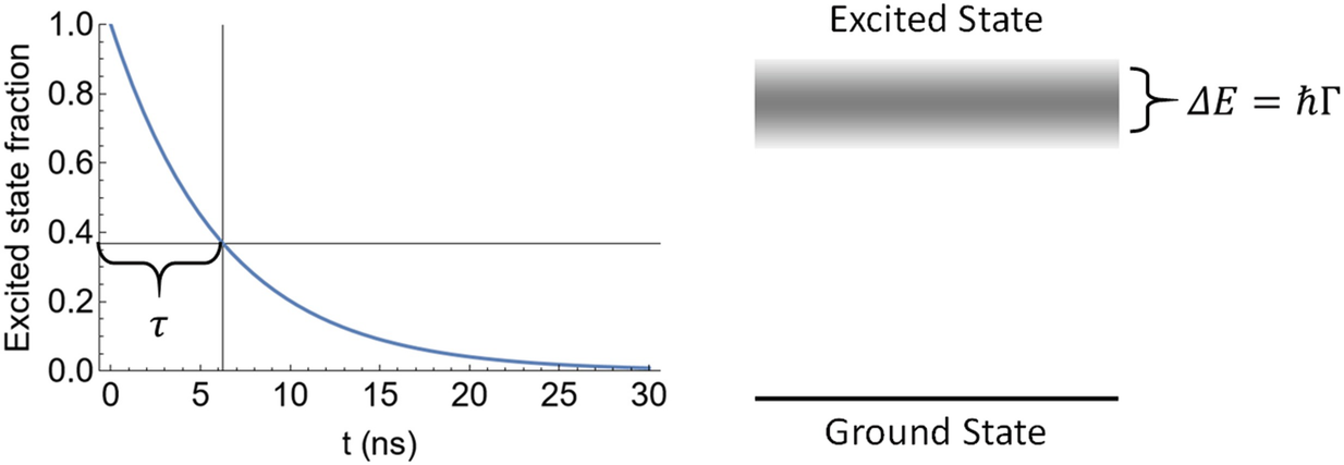
Figure 1:An electron in an excited state decays with a characteristic lifetime . That lifetime is related to the linewidth of the excited state by Eq. (3). If is small, is large. Conversely, if is large, is small
11.3 Antimatter
The Famous Equation
In special relativity, Einstein showed us that energy and mass are the same thing:
This equation is for a particle at rest. If we could somehow convert a proton, which has a mass of , to energy, we would have:
That is a lot of energy![4] This equation also provides us with a brand new unit for mass. The mass of the proton is .
In nature, there are a number of conservation laws that seem to always be true. For example, conservation of energy tells us that for an isolated system (i.e., nothing comes in or out), the total energy of the system is a constant value. Other conserved quantities include charge and angular momentum. As we will discuss in the next section, atom number is not a conserved quantity. For example, we can, and have, created particles from high-energy photons. This process is called pair production. To accomplish this, we send a high-energy photon towards a nucleus. The nucleus “nudges” the photon a little bit and, if the photon has enough energy, it transforms into an electron and a positron.[5] Before the transformation, the photon existed while the electron and positron did not. After the transformation, the photon no longer exists.
A positron, which we introduced at various times throughout the book, is known as the antimatter partner to the electron. It has the same mass and spin as the electron, but it has opposite (positive) charge. Conservation laws are really helpful at telling us the properties of the positron. Since the photon has spin 1 and the electron has a spin of 1/2, conservation of spin tells us the positron also has a spin of 1/2. A photon has no charge. Likewise, the charges of the electron and positron are the same magnitude, but with opposite signs. This is called conservation of charge. Since the photon has no electric charge, if the photon is to be converted into particles, those particles must together have no charge. There are other differences between the electron and positron as well, but we aren’t going to go through all of them.[6] If a positron collides with an electron, the two particles “annihilate” each other back into photons. Before the annihilation, the electron and positron existed while the photons did not. After the annihilation, the electron and positron no longer exist.
Other examples of pair production include creating a muon and an antimuon (see Sect. 11.5 The Standard Model of Particle Physics), a proton and an antiproton, and a neutron and an antineutron. For this book, the exact details of antimatter don’t really matter. What matters is that these antimatter particles can exist, and we have created a lot of antimatter in accelerators or through studying decay. If an antimatter particle collides with its matter partner, they will annihilate each other creating photons.[7]
Fun Fact
The nuclei of an atom can also have excited states similar to the electrons in the atom. These nuclear excited states are much higher energy compared to electron excited states. Almost all of these excited states emit a high energy photon called an x-ray or a gamma ray to transition back to the nuclear ground state. However, there are nuclei that emit matter and antimatter pairs to transition back to the nuclear ground state! As an example, oxygen-16 has an excited state about above the nuclear ground state.[8] When an oxygen-16 nucleus is in this excited state, it would violate conservation of angular momentum if it did decay to the nuclear ground state by emitting a photon. So, instead the nucleon gets rid of the energy by emitting an electron and positron in order for the nucleus to transition back to the nuclear ground state.
11.4 Going from Quantum Mechanics to Quantum Field Theory
11.4.1 Remove the Conservation of Particle Number Constraint
Reminder
Quantum mechanics conserves particle number. However, unstable atoms decay, and we create and destroy particles all the time at particle accelerators.
To fix this incompatibility with nature (i.e., the theory says no, but experiment says yes), physicists had to remove the constraint of conservation of particle number from their models. Particle number is clearly not conserved in nature, so we should try to make a model that doesn’t conserve particle number. However, this causes a really interesting problem. The Schrödinger equation models an individual particle. What do we do if the particle doesn’t always exist? The solution was to form a mathematical model that doesn’t try to model a particle, but something called a field. But what is a field? The easiest way to understand a field is with a few examples. Figure Figure 2 is a temperature field of the minimum temperatures across the Nordic countries Norway, Sweden, and Finland from January 27, 1999. The region had an unusually cold day.[9] For reference, and . This type of field is known as a scalar field. Every point on the map has a temperature. If I told you a coordinate, you could tell me the temperature at that coordinate. In other words, this scalar field is really some function . If you knew the function, you could quickly find the temperature for any coordinate values of x and y.
![A scalar field showing the minimum temperatures across the Nordic countries Norway, Sweden, and Finland on January 27, 1999. The data used to make this plot was taken from the Copernicus Climate Change Service, Climate Data Store, see Reference [1]](/AtomicPhysicsForEveryone/build/541577_1_En_11_Fig2_-5d5d58474e5b6c015676d94efd92f0a3.png)
Figure 2:A scalar field showing the minimum temperatures across the Nordic countries Norway, Sweden, and Finland on January 27, 1999. The data used to make this plot was taken from the Copernicus Climate Change Service, Climate Data Store, see Reference [1]
Figure Figure 3 is another type of field known as a vector field. This is a plot that shows the speed of wind in a simulated tornado. This is, again, a function, but the answer that you get from this function is a vector. It tells you both the speed of the wind and the direction. Other vector fields you might have heard about are electric fields and magnetic fields.
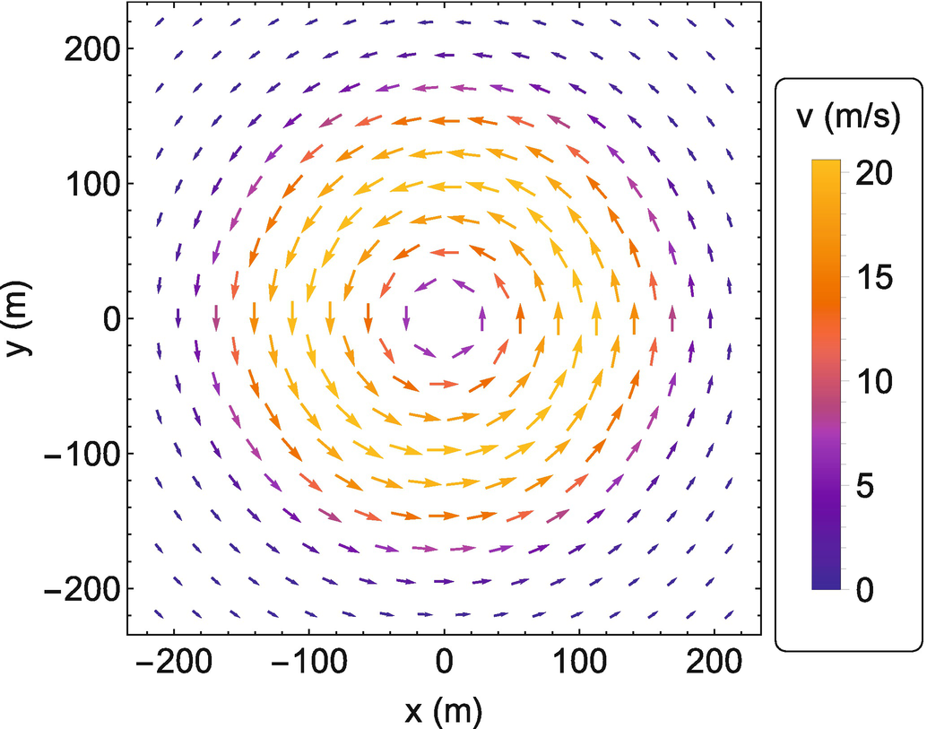
Figure 3:A (simulated) vector field showing the wind speed of a tornado that has a diameter of about 300 m and a top speed of about 20 m/s. This type of plot gives us both direction (the flow is counterclockwise) and the speed of the air
Instead of following around a particle, quantum field theory keeps track of a field. Particles are “excitations” of the fields. As an analogy, let’s think about the standing waves on a quantum mechanical string, see Fig. Figure 2. The background field in this analogy would be the state with a single loop. The particle would be an excitation of this field, or the state with two loops. A quantum particle can go into the field (in our analogy, the system went from two loops to one) or come out of it (one loop to two). Consider a free neutron moving through space. We know from Chap. 10. Isotope Shifts, Radioactive Decay, and the Nuclear Forces that a free neutron is unstable and will decay into a proton, an electron, and an anti-electron neutrino with a half-life of about 11 minutes. From a mathematical viewpoint, that neutron is described as moving through a quantum field. When the neutron decays, the neutron goes into the field and a proton, electron, and anti-electron neutrino come out of the field.[10]
Important Summary
Removing the constraint on conservation of particle number forced physicists to develop a model that doesn’t rely on a particle always existing. Instead, quantum field theory models fields where particles can go into or out of these fields.
11.4.2 Vacuum Fluctuations
Vacuum fluctuations are temporary changes in the energy of a point in space due to the energy-time uncertainty principle, Eq. (2). Removing the constraint on conservation of particle number combined with the energy-time uncertainty principle, results in bizarre behavior. Quantum field theory predicts that particles are continually popping out of and returning into the field. Interestingly, this behavior is not forced; it naturally comes from removing conservation of particle number and including the energy-time uncertainty principle in the model! As a rough analogy, quantum field theory says these particles are excitations of fields similar to exciting a standing wave from one mode to another. This excited state will not last forever, but decay back into the field after a characteristic time .
Think about that for a moment. According to quantum field theory, there is no such thing as empty space. Space is constantly being filled with particles that pop out of and decay back into fields. This might disturb you a bit. Einstein’s famous equation says that . Reading this equation, we would say that mass and energy are the same thing just like laser frequency, wavelength, and photon energy are all the same thing.
So, doesn’t this violate conservation of energy? Particles that have mass are popping out of the field. Mass is energy, so energy that didn’t exist now exists. However, the energy-time uncertainty principle actually allows nature to seemingly violate conservation of energy, but only for a very short amount of time. The more massive the particle that pops into existence (a big ), the quicker that particle must return to the field (a small ). Removing conservation of particle number combined with the energy-time uncertainty principle allows this odd behavior to happen. It is important to reiterate that this behavior is a natural consequence and not something forced into the math. The temporarily existing particles are known as virtual particles.
These fluctuations can be used to explain why an electron in an excited state decays back to the ground state. These virtual particles, when they exist, push on the atom from the outside. This is the external interaction that causes the electron to fall back to the ground state. Remarkably, theorists can use these vacuum fluctuations to calculate the lifetime of an excited state, and their math correctly predicts the lifetime of excited states.
These virtual particles also explain why the mass of a proton or neutron is so much heavier than the three quarks that make them up. Inside the proton (or neutron), the three quarks are bound tightly together by the strong nuclear force, mediated by virtual particles known as gluons. We will discuss quarks and gluons more in Sect. 11.5 The Standard Model of Particle Physics. Because of this strong binding, quantum field theory predicts that virtual particles are continuously generated and annihilated within the field. The time-averaged mass of the proton thus includes not only the mass of the three quarks but also the contributions from these virtual particles. Ready to have your mind blown: 99% of the mass of a proton (or neutron) comes from particles popping into and out of the field. That means that 99% of your mass has now gone back into the field and been replaced with new particles from the field.[11]
I recognize that this all probably seems very, very odd. But, every experiment seems to confirm that these surprising predictions are true.
11.4.3 Speed of Causality and Feynman Diagrams
Einstein’s theory of special relativity put a speed limit on the universe. Nothing, including information, can travel faster than the speed of light. However, the Schrödinger equation has instantaneous information transfer. How do we solve this problem of instantaneous information transfer?
The answer is force carriers. These force carriers are particles that temporarily come from the field to transmit information from one particle to another. These ideas are nicely illustrated in Feynman diagrams, which are named after the American physicist Richard Feynman.
How to read a Feynman diagram:
Time goes from the bottom to the top.[12] The horizontal axis looks like it should describe a spatial coordinate, but it doesn’t. The horizontal axis doesn’t really mean anything.
Particles are represented using straight lines with arrows on them. Matter has arrows that point in the same direction as time (up) while antimatter has arrows that point in the opposite direction as time (down).
Force carriers are wavy lines.
Particle creation and annihilation occur at the vertices.
A Feynman diagram is not just a wonderful way to visualize a quantum mechanical process. Each diagram is actually a visual representation of a complicated mathematical equation from quantum field theory. An example Feynman diagram can be seen in Fig. Figure 4. In this Feynman diagram, we have two electrons that exchange a “virtual photon,” which can exist for a short amount of time because of the energy-time uncertainty principle. That virtual photon comes from the field and does not exist for very long before returning to the field.
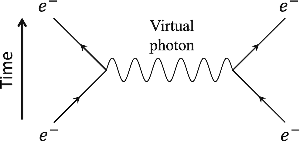
Figure 4:An example of a Feynman diagram. This diagram illustrates a possible interaction between two electrons
The virtual photon transmits information, including the electromagnetic force, from one electron to the other electron. This is how quantum field theory describes the Coulomb interaction! When two electrons are close to each other, the virtual photons that mediate the electromagnetic force between them can exist for a short time due to the energy-time uncertainty principle. Since the virtual photons don’t have to exist for a very long time, they can have higher energy, resulting in a strong repulsive interaction between the like charges. As the two electrons move further apart, the virtual photons need to exist for a longer time to mediate the interaction, which means they have less energy. Consequently, the force between the two charged particles decreases with distance. This is why, according to quantum field theory, the repulsive or attractive force between two charged particles diminishes as the distance between them increases.
Other things can happen as well. For example, Fig. Figure 5 describes how a virtual photon can split into an electron-positron pair when traveling between the two charged particles. This doesn’t happen very often compared to the simple exchange of a virtual photon (the electron-positron pair have much more energy, so the energy-time uncertainty principle makes it harder for this to happen), but when the electron-position pair pop into existence from the field, they have a real impact on the system.
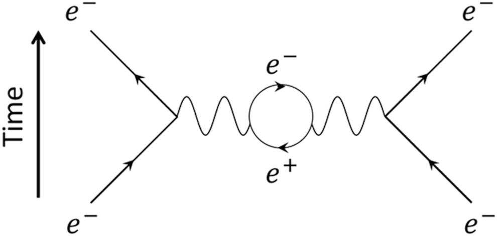
Figure 5:A Feynman diagram depicting how a virtual photon can momentarily split into an electron-positron pair while being exchanged between two electrons
Consider an electron in an atom. That electron is constantly interacting with the protons in the nucleus via virtual photons. Every once in a while, that virtual photon breaks apart into an electron-positron pair similar to Fig. Figure 5 (just replace one of the electrons with a proton). The effect of the electron-positron pair is that the transition frequency between any two states is shifted by just a little bit, but this small shift is still big enough for us to experimentally measure!
There are other things besides virtual photons and electron-positron pairs that can happen, and theorists calculate the effect that all of these different scenarios will have on an atom. Adding up all of the different possible scenarios produces a single overall shift to the transition frequency. Experimentalists then go measure the transition frequency.
Quantum field theory uses all these ideas to make predictions about the atom. Remarkably, these predictions have almost always been confirmed by experiment. In fact, the theory has been confirmed so many times that if there is a disagreement between theory and experiment, we all assume someone made an error.
There are two major subfields to quantum field theory: quantum electrodynamics and quantum chromodynamics. Quantum electrodynamics (QED) is a mathematical framework that describes interactions between charged particles and light (including virtual photons). Quantum chromodynamics (QCD) is a mathematical framework that describes the interactions inside the nucleus including the interactions of the quarks inside the proton and neutron.
11.4.4 One More Thing
You may have heard some form of the expression, “Particle accelerators make particles.” This is a true statement, but we now have the background to understand how they make new particles. According to quantum field theory, we have virtual particles popping into existence from the field and hanging out for a short amount of time before returning to the field.
Important Reminder
Einstein showed us that energy and mass are the same thing
Let’s take two protons and give them a ton of kinetic energy. Next, we are going to smash the two protons together. If the kinetic energy of the protons is larger than the energy equivalent of the particle’s mass coming from the field (), the production of that particle does not violate conservation of energy. In this case, the energy-time uncertainty principle is not the limiting factor, allowing the particle to exist as a real particle. This is exactly what particle accelerators do. Almost all of the particles created in accelerators are unstable and undergo radioactive decay, but they exist long enough for us to determine important properties of the particles, such as mass, charge, and spin.
11.5 The Standard Model of Particle Physics
Quantum field theory is currently the best mathematical model that we have to describe the world of the super small. The conceptual model is called the Standard Model of Particle Physics, or just the Standard Model for short, see Fig. Figure 6.
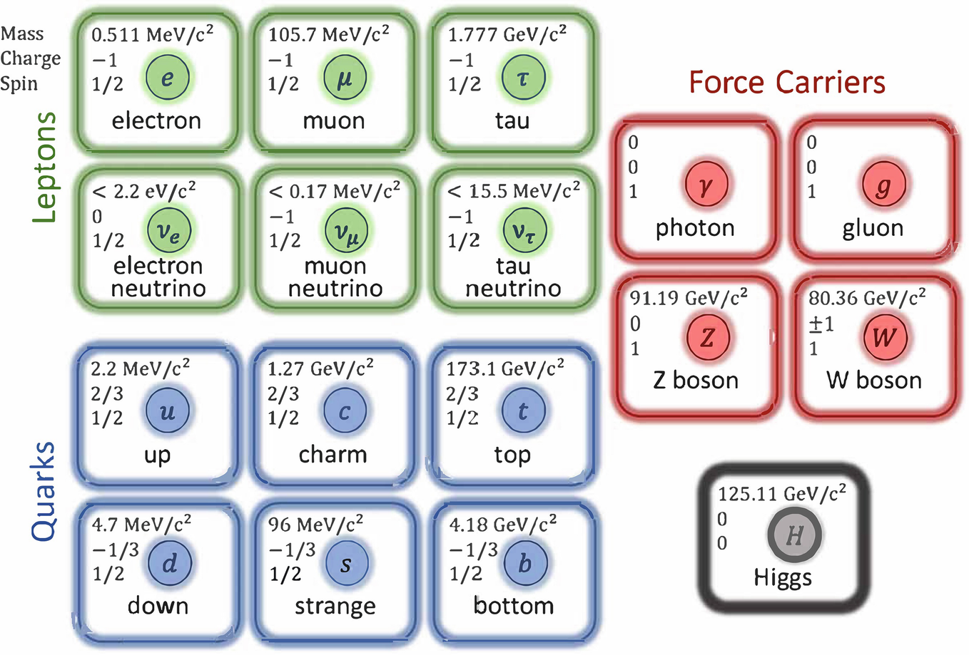
Figure 6:The standard model of particle physics
A Little History
Before the 1960s, the world of particle physics was really confusing. Physicists at particle accelerators were creating hundreds of new particles. It was a little overwhelming; could there really be hundreds upon hundreds of elementary particles? There were so many new particles that in 1956, an American physicist named Robert Oppenheimer coined the term “subnuclear zoo.”
In 1964, American physicists Murray Gell-Mann and George Zweig independently realized that the whole crazy picture could be simplified to just a few elementary particles: quarks. Despite particle accelerators seemingly finding new particles almost every week, what they figured out was that all of the particles were made from twelve elementary particles and their antimatter counterparts. Six of these are now called the up quark, the down quark, the charm quark, the strange quark, the top quark, and the bottom quark,[13] and all of their antimatter counterparts.
At the moment, our best conceptual model of the world of the super small says that everything in the universe is made up of the elementary particles shown in Fig. Figure 6. There are four major groupings in the Standard Model.
Leptons are elementary particles that do not experience the strong force and include electrons, muons, taus, neutrinos, and all their antimatter counterparts. They are colored green in Fig. Figure 6.
Quarks are elementary particles that experience all fundamental forces, including the strong force. Each quark has an antimatter counterpart. Any particle made from quarks, including protons and neutrons, is called a hadron. They are colored blue in Fig. Figure 6.
Force Carriers are particles that mediate the fundamental forces. They include the photon (electromagnetic force), W and Z bosons (weak force), gluons (strong force), and the hypothetical graviton (gravity). They are colored red in Fig. Figure 6.
Higgs Boson is an elementary particle associated with the Higgs field, which gives mass to other particles. It is colored black in Fig. Figure 6.
Protons are composed of 2 up quarks and 1 down quark. A neutron is made up of 1 up quark and 2 down quarks. Helium-4, which has 2 protons, 2 neutrons, and 2 electrons, is actually made up of 6 up quarks, 6 down quarks, and 2 electrons. All of the particles from the subnuclear zoo were made from the six quarks and their antimatter partners. For example, one of the many particles from the zoo is known as the charmed sigma particle, which is actually composed of 2 up quarks and 1 charm quark. Another particle from the zoo is the pion, which is composed of 1 up quark and 1 anti-down quark (the antimatter version of the down quark).
The four elementary particles colored red are the force carriers. Even though the gluon is listed once, there are actually 8 different types of gluons. All 8 of them are carriers for the strong force, which transmit information between quarks. The photon is the force carrier that transmits information between charged particles. Finally, the Z boson and the two W bosons are force carriers for the weak nuclear force, which is the force responsible for decay, decay, and electron capture. Also, notice how massive the W and Z bosons are. This is why the weak force is such a short range force. The uncertainty principle tells us that those force carriers simply can’t exist for very long making their range very, very short.
We can now be more precise in what happens during decay, see Fig. Figure 7. During this process, a down quark in the neutron is transformed into an up quark, resulting in the neutron becoming a proton. This transformation is facilitated by the emission of a boson, which quickly decays into an electron and an anti-electron neutrino. The proton remains in the nucleus, while the electron and anti-electron neutrino are emitted from the atom.
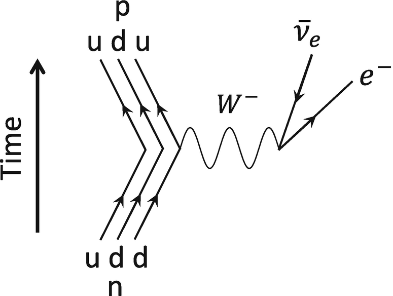
Figure 7:A Feynman diagram showing how a neutron decays into a proton. A neutron is composed of 2 down quarks and 1 up quark. One of the down quarks is transformed into an up quark. This transformation is facilitated by the emission of a boson, which quickly decays into an electron and an anti-electron neutrino
Once again, I admit that all of this seems a little …out there. But everything we have talked about so far really just naturally falls out of the math when we remove or add the restrictions that we talked about in Sect. 11.1 Problems with Quantum Mechanics. More importantly, the math behind this conceptual model seems to do an amazing job both modeling and predicting the world of the super small.
The final fundamental particle in the Standard Model is the Higgs boson, named after British physicist Peter Higgs. Simply put, the Higgs field interacts with all particles that have mass. Particles with mass are constantly interacting with the Higgs field through the Higgs boson. This interaction is, according to the Standard Model, the thing that gives the particles mass. This was the last particle to be discovered by particle physicists. The Higgs boson itself was theoretically predicted back in 1964 and finally created in a particle accelerator in 2012. Peter Higgs and Belgian physicist François Englert won the Nobel Prize for the Higgs boson in 2013.
11.6 So, What’s Next?
This is exactly the question physicists are always asking! We want to understand nature. To do so, we develop models and test the models to make sure they accurately describe nature. There are different ways to test the Standard Model, and Part 1 of this book discusses how atomic and nuclear physicists use spectroscopy as a tool to test these models. The Standard Model of Particle Physics, which is mathematically described by quantum field theory, is our current best model for the world of the super small. The theory has been tested over and over again, and it has succeeded almost every single time. However, we know the theory is not complete. There are plenty of things in the universe that are not included in the Standard Model. That means that we might be able to create a more complete theory. Here is a list of some of the phenomena that are not in the Standard Model.
Gravity
Believe it or not, quantum field theory does not include gravity. Einstein’s theory of general relativity is our best model of gravity. General relativity has predicted fascinating phenomena such as gravitational lensing (the theoretically predicted and experimentally measured phenomenon of light bending around massive astronomical objects like large stars and galaxies) and gravitational waves (the theoretically predicted and experimentally measured phenomenon that creates “ripples” in space when two black holes merge; quite literally space is compressed just a little bit and this compression wave ripples out to be detected on earth). Like quantum field theory, general relativity is an incredibly successful theory. Interestingly, the two theories are incompatible with one another. There are a number of reasons why, but one of the big reasons is that general relativity requires “spacetime” to be smooth and continuous while quantum field theory discretizes the fields. In other words, quantum says no to smooth and continuous while general relativity says no to discrete and bumpy. Quantum field theory also needs a force carrier to transmit gravitational information between two objects with mass, which we call a graviton. However, we have yet to create and measure a graviton in the lab.
Where Is All the Antimatter?
Quantum field theory predicts there should be about equal parts matter and antimatter. For example, Fig. Figure 8 shows a photon that has enough energy to create particles (we have done this at accelerators!). The particles that are created are always a matter/antimatter pair. However, when we look out in the universe, we only see matter. So, where is all the antimatter? We don’t know. This problem is called baryon asymmetry. This isn’t a bad thing. If the universe was equal parts matter and antimatter, they would have annihilated each other. So, in a way, this is one experimental measurement that the Standard Model failed to predict. The Standard Model predicts equal amounts of matter and antimatter, while observations show a universe dominated by matter.
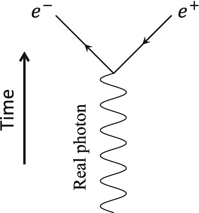
Figure 8:Everything we have done in the lab produces equal amounts of matter and antimatter, like this photon making an electron and a positron
Why Do Neutrinos Have Mass?
This one is short. The Standard Model says that neutrinos don’t have mass. However, they do. This is why I use the phrase “The theory has been tested over and over again, and it has succeeded almost every single time.” The Standard Model says neutrinos don’t have mass, but we have found that they do.
What Is Dark Matter and Dark Energy?
This one is also short. From astronomical observations, the universe is thought to be about 5% atoms, 26% dark matter, and 69% dark energy. However, we don’t even know what dark matter or dark energy is …so it is a little hard to include them in a model. Still, it is kinda weird that our most successful model ever tested (quantum field theory) doesn’t know how to deal with 95% of the universe.
Even though quantum field theory has been incredibly successful, there is still a lot to learn! For physicists, this is the best thing ever. There have been some incredibly interesting and ingenious ideas to make the Standard Model more complete. Some of these ideas include string theory, supersymmetry, and loop quantum gravity. However, no one has come up with any way to definitively test if any of these ideas are correct. But this is what makes everything so exciting! We still have more to learn, more to understand, and more to explore. To learn more and push our understanding always onward, we use the most important equation in all of physics:
11.7 Problems
Fun Fact
The Tevatron was a particle accelerator at Fermi National Accelerator Laboratory (Fermilab), located in Batavia, Illinois, near Chicago. It accelerated protons and antiprotons to energies of 980 GeV, producing proton-antiproton collisions with energies of up to 1.96 TeV. Sadly, the Tevatron shut down in 2011 because the Large Hadron Collider (LHC) at CERN, which became operational in 2008, surpassed the Tevatron in terms of energy levels. The LHC can collide protons at energies of 7 TeV per beam (14 TeV in total). CERN is located in Geneva, Switzerland, and it is currently the world’s largest particle accelerator. CERN is an acronym for the French name “Conseil Européen pour la Recherche Nucléaire,” which translates to “The European Organization for Nuclear Research.”
References
Tveito, O.E., Førland, E.J., Heino, R., Hanssen-Bauer, I., Alexandersson, H., Dahlström, B., Drebs, A., Kern-Hansen, C., Jónsson, T., Vaarby-Laursen E., Westman, Y.: Nordic Temperature Maps DNMI Klima 9/00 KLIMA. Norwegian Meteorological Institute, Oslo (2000). Copernicus Climate Change Service, Climate Data Store, (2021): Nordic gridded temperature and precipitation data from 1971 to present derived from in-situ observations. Copernicus Climate Change Service (C3S) Climate Data Store (CDS). Copernicus Climate Change Service (2021), Accessed Jan 25, 2024
By very fast, we mean something like 10% of the speed of light or faster.
This is also called conservation of probability.
At least you should. It is super important to always know the limitations of your model.
Converting mass to energy is the basic idea behind nuclear reactors.
The nucleus is the external interaction needed to start the process. As a general rule, you always need something acting on the system to initiate such a process.
If you’d like to explore more differences, search the internet for parity. Parity is a concept that is easy to say but hard to understand. Electrons and positrons have opposite parity. Fun fact: we used to think parity was a conserved quantity. However, in 1956, Chinese American physicist Tsung-Dao Lee and Chinese physicist Chen-Ning Yang proposed a theory that the weak force does not conserve parity. This idea was experimentally confirmed by Chinese American physicist Chien-Shiung Wu and her collaborators.
For completeness, other particles besides photons can also be created during annihilation.
For comparison, a 450 nm wavelength photon has an energy of 2.75 eV. So, this nuclear excited state has over 2 million times more energy!
Det här är för kallt!
To be completely correct, only a quark inside the neutron goes into the field and another quark comes out, but we haven’t talked about quarks yet.
For completeness, there are other ways to think about this extra mass. Some physicists prefer to use something called binding energy or simply “fluctuations of the field” to account for the extra mass. All of these ideas are mathematically correct. I have found that virtual particles are a very accessible way for first-time learners to think about the world of the super small. They will also be helpful when we get to force carriers, which are virtual particles, in the next section.
Some physicists like to rotate their Feynman diagrams so that time goes left to right instead of bottom to top.
Some of these names are odd, but it was the 1960s and 1970s .
- Copernicus Climate Change Service. (2021). Nordic gridded temperature and precipitation data from 1971 to present derived from in-situ observations. ECMWF. 10.24381/CDS.E8F4A10C