A “beam” of light is very familiar. A laser pointer, for example, produces a pattern of light that is almost like a transverse section of a plane wave. But not quite. The laser beam spreads as it travels. You might think that this is simply due to the imperfections in the laser. But, in fact, no matter how hard you try to perfect your laser, you cannot avoid some spreading. The problem is “diffraction.”
Interference is a crucial part of the physics of diffraction. We have seen it already in one-dimensional situations such as interferometers and reflection from thin films. Here we begin to see what amazing things it does in more than one dimension.
13.1: Interference
Double Slit
The classic arrangement of the double slit experiment is illustrated in Figure 13.1. There is an opaque screen with two narrow slits in it in the plane (shown in cross section in the plane — the slits come out of the paper in the direction) a small distance apart. The opaque screen is illuminated by a “point” source of light. For example, this could be a light with a clear glass bulb and a colored filter to pick out a narrow frequency range, far away in the − direction. A laser beam spread out with a lens would serve just as well. The important thing is to produce illumination at the opaque screen in which the frequency is in a narrow range and the phase of the light reaching the two slits is correlated. This will certainly be true if the illumination for is nearly a plane wave.
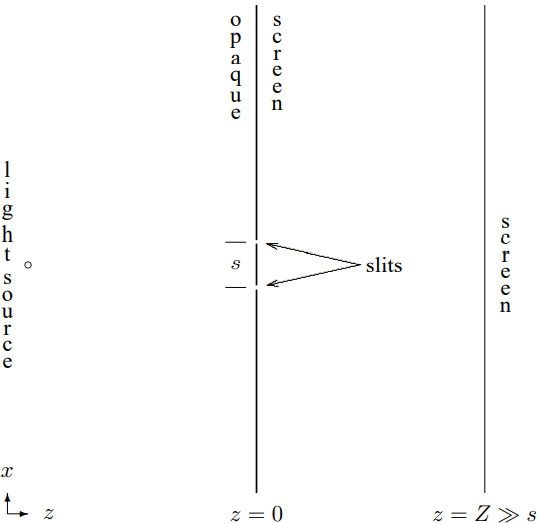
Figure 13.1:The double slit experiment.
Now an interesting thing happens at the second screen, at . This “screen” could be a photographic plate, a translucent screen, or even your retina. What appears on this screen is a series of parallel lines of brightness in the direction (parallel to the slits). If one of the slits is covered up, the lines disappear.
What is going on is interference between the two possible straight-line paths by which the light can reach the screen. We will give a heuristic, physical discussion of the interference in this section. Then in the next section, we will derive the same result using the kind of forced oscillation and boundary condition arguments that you know from our study of one-dimensional waves.
The physical picture is this. The electric field at is a sum of the fields that come from the two slits. At , in the symmetrical arrangement shown in Figure 13.1, the two possible paths for the light have the same length. Therefore, the two components of the field have the same phase. Therefore they interfere “constructively” and there is a bright line at . As x changes, at , the relative length of the two paths changes. We will then get alternating positions of constructive and destructive interference. This gives rise to the bright lines.
We can understand the effect quantitatively by computing the path length explicitly. Consider a point on the screen at . This is shown in Figure 13.2.
The length of the dotted line in Figure 13.2 is
For the upper and lower slits, the path lengths are slightly shorter and longer respectively. The total difference in path length is
For , we can expand in 13.2 in a Taylor series,
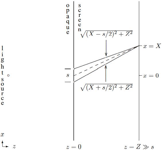
Figure 13.2:Path lengths.
Therefore if the angular wave number of the light is k, the phase difference between the two paths is
We get an intensity maximum every time the phase is a multiple of , when
In terms of the wavelength, , this is
Fourier Optics
Suppose that instead of a simple pattern of two slits, there is some more complicated pattern on the opaque screen. In general, we can describe the wave disturbance in the plane by some function of and
Our strategy will be to think of the wave produced for by this general function as a sum of the effects of tiny holes at all the values of and for which is nonzero. For each little piece of the function, we can compute the path length to some point on the screen at . Then we can add up all the pieces.
Suppose, for simplicity, that is only nonzero in some small region around the origin, so that and will be small
for all relevant values of and . Now the path length from the point on the screen at to the point on the screen at is
Using 13.8, we can expand this as follows:
where
and
Thus the wave on the path from to gets a phase of approximately
Now we can put the pieces of the wave back together to see how the interference works at the point . We just sum over all values of and , with a factor of the phase and the function, . Because and are continuous variables, the sum is actually an integral,
As we will see in more detail below, this is a two-dimensional Fourier transform of the function, .
The equation, 13.14, is the fundamental result of Fourier optics. It contains much of the physics of diffraction. We have made a number of assumptions in deriving it that need further discussion. In the next section, we will derive it in a different way, treating the wave for as the result of a forced oscillation, produced by the wave in the plane. This will give us an alternative physical description of diffraction. But it will be useful to keep the simple picture of adding up all the possible paths in mind as we get deeper into the phenomena of interference and diffraction.
1We are ignoring polarization.
13.2: Beams
Making a Beam
Consider a system with an opaque barrier in the plane. If it is illuminated by a plane wave traveling in the + direction, the barrier absorbs the wave completely. Now cut a hole in the barrier. You might think that this would produce a beam of light traveling in the direction of the initial plane wave. But it is not that simple. This is actually the same problem that we considered in the previous section, 13.7-13.14, with the function, , given by
where
In fact, it will be useful to think about the more general problem, because the the function, 13.16, is discontinuous. As we will see later, this leads to more complicated diffraction phenomena than we see with a smooth function. In particular, we will assume that is signifigantly different from zero only for small x and y and goes to zero for large and . Then we can talk about the position of the “opening” that produces the beam, near .
We can think of this problem as a forced oscillation problem. It is much easier to analyze the physics if we ignore polarization, so we will discuss scalar waves. For example, we could consider the transverse waves on a flexible membrane or pressure waves in a gas. Equivalently, we could consider light waves that depend only on two dimensions, and , and polarized in the direction. We will not worry about these niceties too much, because as usual, the basic properties of the wave phenomena will be determined by translation invariance properties that are independent of what it is that is waving!
Caveats
It is worth noting that there are other approaches to the diffraction problem besides the ones we discuss here. The physical setup we are considering is slightly different from the standard setup of Huygens-Fresnel-Kirchhoff diffraction, because we are studying a different problem. In Huygens-Fresnel-Kirchhoff diffraction,[1] you consider the diffraction of a plane wave from a finite object, whereas, our opaque screen is infinite in the - plane. In the Huygens-Fresnel case, the appropriate boundary condition is that there are no incoming spherical waves coming back in from infinity toward the object that is doing the diffracting. The diffraction produces outgoing spherical waves only. We will not discuss this alternative physical setup in detail because it leads deeper into Bessel functions[2] than we (and probably the reader as well) are eager to go. The advantage of our formulation is that we can set it up entirely with the plane wave solutions that we have already discussed. We will simply indicate the differences between our treatment and Huygens-Fresnel diffraction. For diffraction in the forward region, at large z and not very far from the z axis, the diffraction is the same in the two cases.
The reader should also notice that we have not explained exactly how the oscillation, 13.15,
in the plane is produced. This is by no means a trivial problem, but we will not discuss it in detail. We are concentrating on the physics for . This will be quite interesting enough.
Boundary at 
To determine the form of the waves in the region (beyond the barrier), we need boundary conditions both at and at . At , there is an oscillating amplitude given by 13.15.[3] At , we must impose the condition that there are no waves traveling in the − direction (back toward the barrier) and that the sodwlutions are well behaved at .
The normal modes have the form
where satisfies the dispersion relation
Thus given two components of , we can find the third using 13.18. So we can write the solution as
where
Note that 13.20 does not determine the sign of . But the boundary condition at does. If is real, it must be positive in order to describe a wave traveling to the right, away from the barrier. If is complex, its imaginary part must be positive, otherwise would blow up as goes to . Thus,
We discussed the physical signifigance of the boundary condition, 13.21, in our discussion of tunneling starting on page 274. There is real physics in the boundary condition at infinity. For example, consider the relation between this analysis and the discussion of path lengths in the previous section. In the language of the last chapter, we cannot describe the effects of the waves with imaginary . However, the boundary condition, 13.21, ensures that these components of the wave will go to zero rapidly for large .
Boundary at 
All we need to do to determine the form of the wave for is to find . To do that, we implement the boundary condition at by using 13.19
and setting
to get 13.15. Taking out the common factor of , this condition is
If is well behaved at infinity (as it certainly is if, as we have assumed, it goes to zero for large and ), then only real and can contribute in 13.23. A complex would produce a contribution that blows up either for or . Thus the integrals in 13.23 run over real k from − to .
13.23 is just a two-dimensional Fourier transform. Using arguments analogous to those we used in our discussion of signals, we can invert it to find .
Inserting 13.24 into 13.19 with 13.20 and 13.21
gives the result for the wave, , for . This result is really very general. It holds for any reasonable .
13.3: Small and Large z
But what do we do with it? The integral in 13.19 is too complicated to do analytically. Below, we will give some examples of how it works by doing the integral numerically. However, for small and for large , the integral simplifies in different ways.
Small 
For sufficiently small , we would expect on physical grounds that we really have produced a beam and projected an image of the function, . To see this explicitly, we will use the fact that for a particular (well behaved) , the Fourier transform is a function that goes to zero for
for some much larger than the wavelength. The distance is determined by the smoothness of . Typically, is the size of the smallest important feature in , the smallest distance over which changes appreciably. We saw this in our discussion of Fourier transforms in connection with signals in Chapter 10. We will see more examples below. We can expand in the exponential in a Taylor expansion,
Because of 13.25, the largest value of that we need in the integral, 13.19
is of order . For much larger values, the integrand is zero. Thus the largest possible value of the second term in the expansion 13.26 that matters in the integral, 13.19 is of the order of
Therefore, if is finite and is small , the second term is small and we can keep only the first term, . Then putting this back into the integral, 13.19, we have
This is just what we expect — a beam with the shape of the original function, propagating in the direction with velocity .
The result 13.28 begins to break down when the next term in the Taylor series, 13.26, becomes important. That is when
Thus
marks the transition from a simple beam to the onset of important diffraction effects.
If , which is the situtation in the example of a single slit of width , that we will analyze in detail later, important diffraction effects start immediately because the slit has sharp edges. However, the beam maintains some semblance of its original size until .
For z larger than , the and dependence from the factor cannot be ignored. In general, the evaluation of the integral, 13.19, is very hard. However, for very large , we can use a physical argument to find the result of the integral, 13.19.
Large 
Suppose that you are very far away, at a point ,
Then you cannot see the details of the shape of the opening or other details of , only its position. The wave you detect at some far-away point must have come from the opening and if you are far enough away, it is almost a plane wave. This is called “Fraunhofer” or “far-field” diffraction. If this condition is not satisfied, the problem is called “Fresnel” or “near-field” diffraction. For the light to actually reach your eye in the far-field situation, the propagation vector must point from the opening to you. The situation is depicted in the diagram in Figure 13.3. In the near-field region, the spreading due to diffraction is of the same order as the size of the opening. For much larger , in the far-field region, the vector must point back to the opening.
Thus the only contribution to the integral, 13.19,
that counts is that proportional to where points from the opening to your eye. Because the integrand in 13.19 has a factor of, the amplitude of the wave is proportional to where
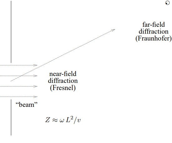
Figure 13.3:The basic diffraction problem — making a beam.
The amplitude is also inversely proportional to
because the intensity must fall off as , as in a spherical wave, by energy conservation.
There are other factors that contribute to the variation of the amplitude besides (we will see one below). However, typically, all the other factors are very slowly varying and can be ignored. Thus we expect that the intensity for large is approximately
where and are related by 13.32.
which implies
or
Now here is the point! Inserting 13.36 into 13.24
gives the integral in 13.14 that came from our physical argument about interference!
Thus our description of the wave for as a forced oscillation problem contains the same factor that describes the interference of all the paths that the wave can take from the opening to . The advantage of our present approach is that it is a real derivation.
We can also write this result in terms of angles:
where and are the angles of the vector from the line in the and directions. Or equivalently,
This is illustrated in the diagram in Figure 13.4.
Stationary Phase
Mathematically, 13.32
arises for large becasue the phase of the exponential in 13.19
is very rapidly varying as a function of and except for special values of and where the derivatives of the phase with respect to and vanish. If the function is centered at and is smooth,[4] the derivatives of are of order and are
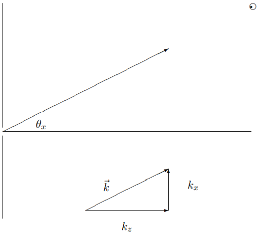
Figure 13.4:irrelevant. Thus the contribution comes from , such that
which is equivalent to 13.38. A careful evaluation of the integral, taking account of the and dependence in the neighborhood of the critical value determined by 13.38 yields an additional factor in the amplitude of the wave of
where is the angle of the vector to the axis. We expected the factor because of the spreading of the diffracted wave with distance. The factor of is actually the only place where the details of the boundary condition at infinity, 13.21, enter into our expression for the diffracted wave. This factor guarantees that the diffracted wave vanishes as we go to the surface of the opaque screen far from the opening. This is analogous to the “obliquity” factor , in the Fresnel-Kirchhoff diffraction theory. The difference between the two is due to the different boundary conditions (our infinite flat barrier versus the lack of incoming spherical waves). We will usually ignore this factor, and indeed it generally does not make much difference where diffraction is important in the forward direction. The important thing is that everything else about the diffraction in the far-field region is determined just by linearity, translation invariance and local interactions.
Spot Size
A useful way to think about the transition from near-field (Fresnel) to far-field (Fraunhofer) diffraction is to consider the size of the spot formed by the beam of Figure 13.3 as a function of . This is a competition between two effects. Increasing the size of the opening makes the spot size larger at small . However, decreasing the size of the opening increases the spread in , thus increasing the diffraction, and making the spot size larger at large . For a given , the best you can do is to choose the size of your opening so that these two effects are of the same order of magnitude. Suppose that the size of your opening is . Then the spread in is of order . At large , the beam spreads into a cone with an opening angle of order
Thus when
the spreading of the spot due to diffraction is of the same order of magnitude as the size of the opening. We conclude that to minimize the spot size for a given , you should choose an opening of size
The relation, 13.41, up to factors of , is what defines the region of Fresnel diffraction in Figure 13.3. Another way of summarizing the result of this discussion is that for
the spreading due to diffraction is much larger than the spreading due to the size of the opening. This defines the region of far-field, or Fraunhofer diffraction.
Angles
What happens if the plane wave in 13.15 is coming in toward the opaque barrier at an angle, rather than head on? To be specific, suppose that the vector of the wave makes an angle with the perpendicular in the - plane, so that
Then it is reasonable to assume that the analog of 13.15, the amplitude of the wave in the plane, is6
where the additional dependence has simply been inherited from the dependence of the incoming wave. We can write the Fourier transform of in terms of that of as follows:
which implies
This is entirely reasonable. If the maximum of occurs at , the maximum of occurs at . Thus the diffraction pattern appears where a line through the opening in the direction of the incoming plane wave crosses the screen, just as we would expect from a skew beam.
13.4: Examples
Single Slit
Suppose
independent of . This is really a two-dimensional problem, because we can keep and ignore it (except for a factor of , that we won’t worry about) by dropping the integral from 13.19. 13.24
becomes (with the corrected to make it one-dimensional)[5]
Thus we expect that the intensity of the wave at large is proportional to ,
where
or
Thus if we measure the intensity of the diffracted beam, a distance from the opening, the intensity goes as follows:[6]
where is the wavelength of the light. A plot of as a function of is shown in Figure 13.5. This is called a diffraction pattern. In the important case of light passing through a small aperture, the diffraction pattern can be easily observed by projecting the diffracted beam onto a screen. The features of this pattern worth noting are the large maximum at , with twice the width of all the other maxima, and the periodic zeros for . Note also that as the width, of the slit decreases, the size of the diffraction pattern increases.
Moral: This inverse relation between the size of the slit and the size of the diffraction pattern is another illustration of the general feature of Fourier transforms discussed in Chapter 10.
Near-field Diffraction
We will pause here to discuss the region for intermediate , Fresnel diffraction, where the diffraction problem is complicated. All we can do is to evaluate the integral, 13.19, numerically, by computer, and find the intensity approximately at various values of . For example, suppose that we take
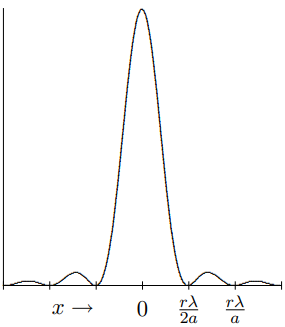
Figure 13.5:The intensity of the diffraction pattern as a function of .
corresponding to a rather small slit, with a width of only times the wavelength of the wave. We will then use 13.19 to calculate the intensity of the wave at various values of , in units of . For small , the result is shown in Figure 13.6. You can see that the basic beam shape is maintained for a while, as we expected from 13.28. However, wiggles develop immediately. The rather large wiggly diffraction is due to the sharp edges. Below, we will give another example in which the diffraction is much gentler. For intermediate , shown in Figure 13.7, the wiggles begin to coalesce and dramatically change the overall shape of the beam. At the same time, the beam begins to spread out.
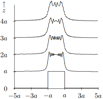
Figure 13.6:The intensity of a wave passing through a slit, for small .
Finally, in Figure 13.8, we show the approach to the large regions, where diffraction takes over completely and the far field diffraction pattern, 13.54, appears.
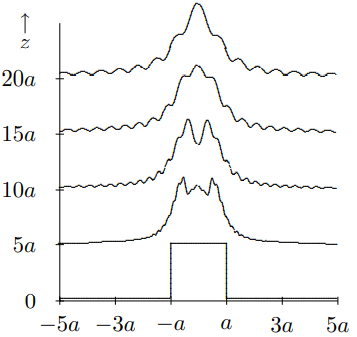
Figure 13.7:The intensity of a wave passing through a slit, for intermediate .
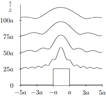
Figure 13.8:The intensity of a wave passing through a slit, as gets large.
One more example may be interesting. Suppose that instead of being a simple hole in the opaque screen, the opening is shaded in such a way that the wave disturbance at has the form
The Fourier transform here was done in Chapter 10 in 10.49-10.56. Substituting and in 10.56 gives
This determines the intensity distribution at large . However, unlike the previous example, this pattern gives very gentle diffraction. For small , the intensity pattern is shown in Figure 13.9. The sharp point in 13.56 disappears, but otherwise the change is very gradual because the initial pattern is very smooth except at . For intermediate and large , the intensity patterns are shown in Figure 13.10 and Figure 13.11.
 for small z.](/physicsOfWaves/build/lt-32780-clipboard_e-f90b035c2359d442d663198b43dca267.png)
Figure 13.9:The intensity distribution from 13.56 for small .
 for intermediate z.](/physicsOfWaves/build/lt-32781-clipboard_e-453e3aeb05c03f9cf5734cb6f9185a09.png)
Figure 13.10:The intensity distribution from 13.56 for intermediate .
 for large z.](/physicsOfWaves/build/lt-32782-clipboard_e-31a472be6fda10ab4b81e2e0381b1abd.png)
Figure 13.11:The intensity distribution from 13.56 for large .
Rectangle
Suppose
This is the product of a single slit pattern in with a single slit pattern in . The Fourier transform is the product of the one-dimensional Fourier transforms
Thus the intensity looks approximately like
Of course, once again, because of the general properties of the Fourier transform, if the rectangle is narrow in , the diffraction pattern is spread out in , and similarly for .
“Functions”
As the slit in 13.49 gets narrower, the diffraction pattern spreads out. Of course, the intensity also decreases. The intensity at is related to the Fourier transform of at zero, which is just the integral of over all . As the slit gets narrower, this integral decreases. But suppose that we increase the intensity of the incoming beam, as decreases, to keep the intensity of the maximum of the diffraction pattern fixed. Ignoring the dependence, we require
The limit of as doesn’t really exist as a function. It is zero everywhere except . But it goes to very fast at , so that
It is extraordinarily convenient to invent an object with these properties, called a “-function”. That is, has the property that it is zero except at , and that
In fact, this object makes a kind of mathematical sense, so long as you do not square it. -functions can be manipulated like ordinary functions, added together, multiplied by constants or smooth functions — -functions of different variables can even be multiplied — just don’t square them! For example, a delta function can be multiplied by an ordinary continuous function:
where the equality follows because the delta function vanishes except at , so that only the value of at 0 matters.
Now it should be clear from 13.63 and 13.64 that the Fourier transform of is just a constant:
The diffraction pattern for this thing is thus very boring. There is uniform illumination at all angles.
Of course, in physics, we can’t make -functions. However, if , in 13.61 is much smaller than the wavelength of the wave, then it might as well be a -function, because it only matters what is for . Larger correspond to exponential waves that die off rapidly with . But for such , the product is very small, thus
and we still get uniform diffraction over all angles.
Moral:-functions are simply a convenience. When physicists talk about a -function, they mean (or at least they should mean) a function like, where is smaller than any physical distance that is important in the problem. Once gets that small, it is often easier to keep track of the math when you go all the way to the unphysical limit, .
Some Properties of -Functions
The Fourier transform of a -function is a complex exponential:
The Fourier transform of a complex exponential is a -function:
A -function can be reached as a limit in a variety of different ways. For example, from 13.68, we would expect that as , the Fourier transform of 13.49 should approach a -function:
Dimension from Two
Using -functions, we can say more elegantly what is meant by the statement we made above that if does not depend on , the problem is one-dimensional. If we look at the limit of 13.58 as , it goes over into 13.49. In other words, when a rectangle is infinitely long, it is a slit. In this limit, the Fourier transform, 13.59 goes into
This is the real meaning of 13.50. It is one-dimensional in the sense that is stuck at 0. There is no diffraction in the direction.
Many Narrow Slits
An interesting application of δ-functions is to the diffraction pattern for several narrow slits. We will use this later in various ways. Consider a function, of the form
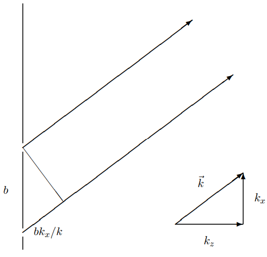
Figure 13.12:If , the interference is constructive.
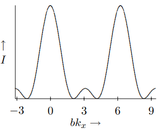
Figure 13.13:The diffraction pattern for three narrow slits.
This describes a series of narrow slits[7] at , , , etc., up to . The Fourier transform of 13.71 is a sum of contributions from the individual -functions,
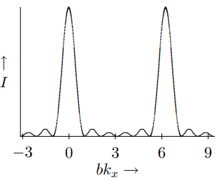
Figure 13.14:The diffraction pattern for 6 narrow slits.
But the sum is a geometric series that can be done explicitly:
Thus the diffraction pattern intensity is proportional to
For , 13.74 is just
This is the problem with which we started the chapter. When for integer , then the wave from one slit travels farther than the wave from the other by , where is the wavelength. Thus for the interference is constructive, as illustrated in figure 13.12.
For larger , we still get constructive interference for , but the maxima are sharper, because with more slits, there are more possibilities for destructive interference at other angles. In Figure 13.13 and Figure 13.14, we plot 13.74 versus from (− to so that you can see two full periods) for and 6. Notice the appearance of secondary maxima between the primary maxima of the intensity. We will return to these relations when we discuss diffraction gratings.
6Again, this is simplistic, ignoring complications from the boundaries in the same way as 13.15.
13.5: Convolution
There is a rather simple theorem, know as the convolution theorem, that is extremely useful in dealing with Fourier transforms. Suppose that we have two functions, and . Define the function as follows:
This integral will be well defined if and fall off fast enough at infinity (and certainly if they are nonzero only in a finite region of ). Note that is a function of a single variable. It is also symmetric under the exchange of the two functions, because by a simple change of variables
Now the theorem is that the Fourier transform of the convolution is times the product of the Fourier transforms of the two functions. The proof is immediate (all integrals run from − to ):
Now we substitute and write the integral over and ,
The two-dimensional analog of 13.79 is a straightforward extension. The two-dimensional convolution is
Repeated Patterns
The convolution theorem can be used to understand many interesting situations. Consider the following very instructive pattern of two wide slits:
for . A piece of the pattern is shown in Figure 13.15 for .
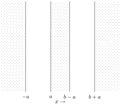
Figure 13.15:A piece of the opaque barrier with two wide slits.
This can be regarded as the convolution of two functions:
where
and
f2(x, y) = δ(x) δ(y) + δ(x − b) δ(y). The corresponding Fourier transforms are, from 13.70 13.84 13.85 Cf1 (kx, ky) = sin(kxa) π kx δ(ky) 13.86 and from 13.73 Cf2 (kx, ky) = 1 4π2 cos bkx 2 e−ibkx/2 . Now applying the convolution theorem gives 13.87 Cf1◦f2 (kx, ky) = cos bkx 2 e−ibkx/2 sin(kxax) π kx δ(ky). 13.88 13.6. PERIODIC f(x, y) 395 Because b > 2a, this describes a pattern that oscillates rapidly on the scale set by 1/b, with an amplitude that varies with the single slit diffraction pattern characterized by size 1/a. The intensity pattern on a distant screen is shown in figure 13.16, for b = 3.5a The dotted line is the pattern for a single wide slit (compare 13.5).
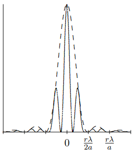
Figure 13.16:The diffraction pattern for two wide slits.
13.6: Periodic f(x, y)
Suppose is periodic in with period . That is
Then can only be nonzero if
To see this, insert 13.89 into 13.24,
If we change variables from , Equation 13.91 is
because the constant phase factor can be taken outside the integral. Equation 13.90 follows because Equation 13.92 implies that either or .
An example of this general principle is Equation 13.74. In the limit that , 13.74 goes to 0 except for for integer (where it is infinite). This example is simple because the slits are narrow, so the intensity is independent of . However, with repeated wide slits, or some more complicated pattern, we could use the convolution theorem and 13.74 to see that 13.90 emerges as . The details of the pattern of each slit will then determine the relative intensity of the diffraction pattern at different .
Thus any infinite regular pattern produces a discrete sequence of ’s. For example, a transmission diffraction grating, that consists of lots of equally spaced lines in the direction with separation on a transparent substrate, produces a that is nonzero only for (because there is no dependence at all) and . Then 13.19 becomes
This describes a linear superposition of plane waves fanning out at angles in the direction given by
as shown in Figure 13.17.
Typically, for a transmission grating, most of the light goes into the central line, which is to say that you can see right through the grating. Note that the even spacing in in 13.94 corresponds to an increasing spacing of the lines projected onto a screen at fixed large (for example, a screen like your retina!) because the distance along the screen is determined by
There is a maximum value of , above which no propagating wave is produced (because it corresponds to and thus imaginary ).
Note also the dependence of 13.94 on wavelength. The larger the wavelength of the light, the larger the angles in the pattern from the diffraction grating. This, of course, is why the diffraction grating is useful. It can separate light of different frequencies. The different colors of the rainbow are spread out along a line, for each value of . This is illustrated in the Figure 13.18, for three frequencies, blue light with wavelength 4300 , green light with wavelength 5200 and red light with wavelength 6300 , incident on a diffraction grating with 10,000 lines per inch. We have shown 13.95 for = −3 to 3 and labeled the colors for the secondary maximum. As you see, in a realistic grating, the angles of diffraction can be large, and it is a very bad idea to use a small angle approximation.
13.6.1 Twisting the Grating
Some interesting examples of the effects discussed in 13.48 occur when the incoming light wave comes at the grating at an angle with respect to the perpendicular. Starting with the
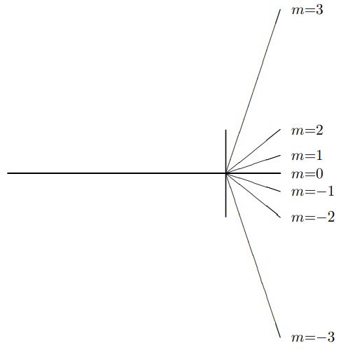
Figure 13.17:A transmission diffraction grating splits a beam of a single frequency.
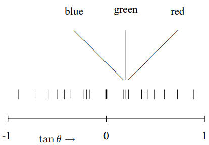
Figure 13.18:The pattern of three frequencies of light from a grating.
grating lines in the direction and the grating in the - plane, there are two different effects.
Twisting Around the Axis
Suppose that the light comes in at an angle from the perpendicular in the - plane. Then from 13.48,
where is Fourier transform for the perpendicular grating,
Thus
or
In other words, is simply displaced by . For example, this means that if , the pattern is exactly the same, but the central maximum has moved over, as shown in Figure 13.19.
Twisting Around the Axis
Suppose that the light comes in at an angle from the perpendicular in the - plane. Then from 13.48.
Now instead of being 0, is fixed at
Now the diffracted waves make nontrivial angles from the perpendicular both in and in
and
Again, as in 13.95, what we see if we project the pattern onto a perpendicular screen at fixed are the tangents,
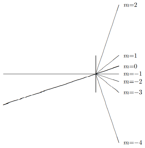
Figure 13.19:The pattern for a beam at an angle, .
where
Thus the diffraction pattern appears curved. What one sees on a screen or a retina is the colors of the rainbow spread out along a curved line. This is shown in Figure 13.20, where we plot versus for a light source and grating as in 13.18, above, but with . Note that the pattern has not only curved, it has spread out, compared to 13.18. Here you really see the three-dimensional vector in action. As increases, for fixed , increases as well, because decreases.
Resolving Power
The discussion so far has assumed that the diffraction grating is truely periodic. But this is only possible if the grating is infinite! In a finite grating, only the middle is periodic. The edges break the periodicity. In a grating consisting of only a finite number of grooves, , the diffraction peaks are not infinitely sharp. They are not delta functions. However, as discussed at the beginning of this section, we actually already know what they look like in the finite
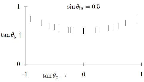
Figure 13.20:The diffraction pattern from a twisted grating.
case because we have solved the problem of diffraction from evenly spaced narrow slits, in 13.74. In the general situation for identical grooves, the intensity looks like 13.74 multiplied by some slowly varying function that depends on the shape of the grooves (by the convolution theorem, 13.79). The important consequence of this is that the shape of a diffraction peak for an -slit grating is roughly given by 13.74.
The shape of the diffraction peak is important for the following practical question. Suppose that you have a beam of light that consists of a superposition of light of two different frequencies. How close together do the frequencies have to be before their nontrivial diffraction peaks melt together, so that you cannot use your diffraction grating to distinguish them? The larger the number of grooves in the grating, the sharper the diffraction peaks and the easier it is to distinguish different frequencies.
Rayleigh’s criterion is an historically important way of answering this question. Rayleigh assumed that it would be possible to distinguish the diffraction maxima from equally intense waves of slightly different wavelengths if the maximum of one frequency coincides with the first minimum of the other. For a grating of 6 lines, this criterion is illustrated in Figure 13.21. The solid line is the total intensity of a wave consisting of two slightly different frequencies. The contributions from the separate frequency components are indicated by the dotted and dashed lines.
Any such fixed criterion for resolving power should be regarded not as a fact about nature, but as a conventional definition that facilitates communication between experimenters. It is always possible to do better than any given definition by accumulating accurate data on the line shape and modeling the details.
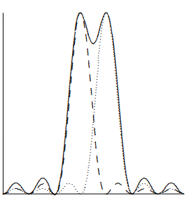
Figure 13.21:Rayleigh’s criterion for a grating with 6 lines.
Blazed Gratings
As a spectroscope, the transmission diffraction grating has a disadvantage compared to a prism. The difficulty is that, as we noted above, most of the light impinging on the grating goes right through and is not split into its component frequencies. This is a very serious problem in devices in which the total amount of light is limited. It is often important to have the bulk of the light going into a single nonzero value of in 13.94. Then nearly all of the photons can be used for the measurement, rather than being wasted in the maximum (which carries no information about the frequency). As we argued above, there is no theoretical reason why such a thing cannot be done. The general principles of translation invariance and local interactions determine the possible angles of diffraction, but not how much light goes to which angle.
In fact, there is a practical and widely used method in reflection gratings. A reflecting surface with a series of evenly spaced parallel lines scored into it acts as a reflection grating, as illustrated in Figure 13.22. This shows a reflection grating in which the predominant reflection of a beam coming in perpendicular to the plane of the grating is also perpendicular. What we want instead is shown in Figure 13.23. To construct such a grating, you can shape the grooves in the grating so that the specular reflection from the individual grooves directs the beam into the nontrivial diffraction maximum, as shown in Figure 13.24.
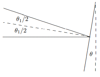
To do this, you can choose the angle of the blaze to be half the angle of the first maximum, , in 13.94, as shown in the blow-up of a groove in figure 13.25.
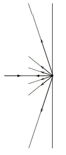
Figure 13.22:A reflection diffraction grating splits a beam of a single frequency.
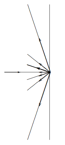
Figure 13.23:A blazed grating directs the beam into a nontrivial diffraction maximum.
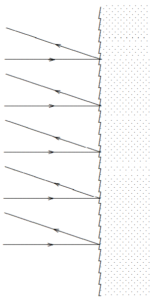
Figure 13.24:The grooves of a blazed grating.
13.7: X-ray Diffraction
A beautiful three-dimensional example of diffraction from a periodic function is x-ray diffraction from crystals. A crystal is a regular array of atoms whose positions can be described by a periodic function
where is any vector from one point on the lattice to another. Mathematically, we can define the lattice as the set of all such vectors. Note that the lattice always includes the zero vector, the point at the origin. The three-dimensional Fourier transform of is nonzero only for wave number vectors of the form
where are the basis vectors for the “dual” or “reciprocal” lattice that satisfies
The idea here is the same as the one-dimensional discussion of the diffraction grating, that , 13.90. The derivation of 13.107 is precisely analogous to that of 13.90.
We can visualize the relation between the lattice and the dual lattice more easily for two-dimensional “crystals.” For example, consider a lattice of the form
shown in Figure 13.26 (for ).
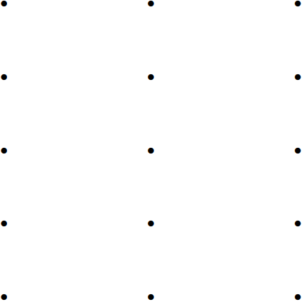
Figure 13.26:A crystal lattice.
It is clear that vectors of the form
satisfy 13.108. Furthermore, a little thought will convince you that these are the shortest pair of linearly independent vectors with this property. Thus we can take 13.110 to be the basis vectors for the dual lattice, so that the dual lattice looks like
as shown in Figure 13.27.Note that the long and short axes are interchanged, as usual in a diffraction process.
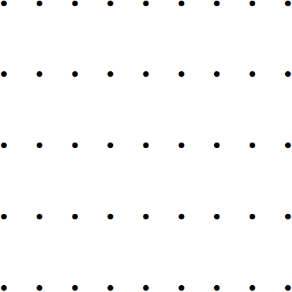
Figure 13.27:The dual lattice.
Now suppose that there is a plane wave passing through the infinite lattice,
The wave that results from the interaction of the plane wave with the lattice then has the form
where is a periodic function, like in 13.106. To find the possible refracted waves, we must write this in the form:
But we also know from the discussion above that the Fourier transform of is nonzero only for values of of the form 13.107. Thus 13.114 takes the form
Therefore, the in 13.114 must have the form
But this is only possible if satisfies the dispersion relation in the material, which means, if the material is rotation invariant so that depends only on , that
Thus we get a diffracted wave only for such that 13.117 is satisfied. X-ray diffraction from a crystal, therefore, can provide direct information about the dual lattice and thus about the crystal lattice itself.
There is a more physical way of thinking about the dual lattice. Consider any vector in the dual lattice that is not a multiple of another,
Now look at the subset of vectors on the lattice that satisfy
This subset is the set of lattice points that lie in the plane, , that is the plane perpendicular to passing through the origin. Now consider the subset
This subset is the set of lattice points that lie in the plane, , that is parallel to the plane , in the lattice. This plane is also perpendicular to and passes through the point (which may not be a lattice point)
Therefore, the perpendicular distance (that is in the direction) between the two planes is
We can continue this discussion to conclude that the subset of lattice points satisfying
is the set of lattice points lying on parallel planes perpendicular to , with adjacent planes separated by . But this set must be all the lattice points! This is true because is an integer for all lattice points by the definition of the dual lattice. Thus all lattice points lie in one of the planes in 13.123.
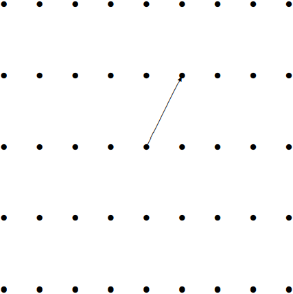
Figure 13.28:A vector in the dual lattice.
These considerations are illustrated in the two-dimensional crystal in the pictures below. If the vector in the dual lattice is as shown in Figure 13.28, then the perpendicular planes in the lattice are shown in Figure 13.29.
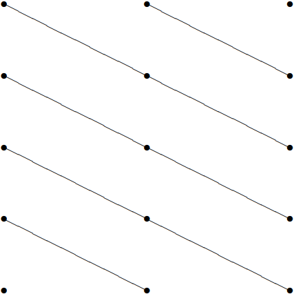
Figure 13.29:The corresponding planes in the lattice.
Now suppose that is one of the special points in the dual lattice that gives rise to a refracted wave, so that
This relation is shown in Figure 13.30. This shows that the vector of the refracted wave, , is just reflected in a plane perpendicular to . We have seen that there are an
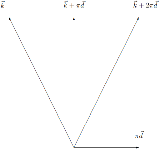
Figure 13.30:The Bragg scattering condition.
infinite number of such planes in the lattice, separated by . The contribution to the scattered wave from each of these planes adds constructively to the refracted wave. To see this, consider the phase difference between the incoming wave, and the diffracted wave for . Evidently, the phase difference at any point is
This phase difference is an integral multiple of on all the planes
Thus the contribution to scattering from all of the planes of lattice points adds constructively, because the phase relation between the incoming and diffracted wave is the same on all of them. Conversely, if , then the contribution from different planes will interfere destructively, and no diffracted wave will result.
This physical interpretation goes with the name “Bragg scattering.” The planes, 13.123 (or 13.126) are the Bragg planes of the crystal. Note that as the vector in the dual lattice gets longer, the corresponding Bragg planes get closer together, but they are also less dense, containing fewer scattering centers per unit area. Generally the scattering is weaker for large .
Problems
13.9: Fringes and Zone Plates
Holographic Image of a Point
One of the simplest of holographic images is the image of a single point. If a plane wave encounters a very small object in its path, the object will produce a spherical wave. If the plane wave and the spherical wave then are absorbed by a photographic plate, as shown in Figure 13.34, an interference pattern is produced in the form of concentric circles, or fringes.
Specifically, suppose that the plane wave is propagating in the direction, the photographic plate is in the - plane at and we put the origin of our coordinate system at the position of the source of the spherical wave, as shown in Figure 13.34. Then the linear combination of plane wave plus spherical wave has the form (ignoring polarization)
where . We will assume, for simplicity, that and are real which means that the two waves are in phase at the object. The intensity of the wave at , on the photographic plate is therefore
where is the distance from the object for a point in the plane,
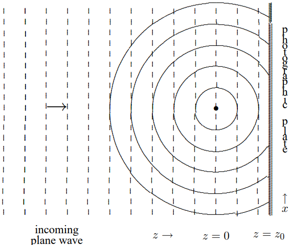
Figure 13.34:Fringes.
and
is the distance from the axis in the - plane. The intensity depends only on , as it must because of the symmetry of the system under rotations around the axis.
Usually, we are interested in the region, , because, as we will see, the intensity pattern is most interesting for small . In this region, the distance, is very nearly equal to . We can ignore the variation of in the amplitude, . However, there is interesting dependence in the cosine term in 13.133. In this term, we can expand in a Taylor series around ,
Putting all this together, the intensity is given approximately for by
The intensity pattern, (13.137), describes concentric circular “zones” of intensity variation. The zones can be labeled by the maxima and minima of the cosine, at
or
where is the wavelength of the wave. For even, the cosine has a maximum and for odd, a minimum. The intensity variation is greatest if the plane wave and the spherical wave have approximately the same amplitude at the plate,
Then the amplitude actually goes to zero at the minima. The intensity distribution as a function of is shown in Figure 13.35. The positions of the maxima and minima, or “zones,” are shown on the axis. On the photographic plate, this intensity distribution gives rise to circular fringes.
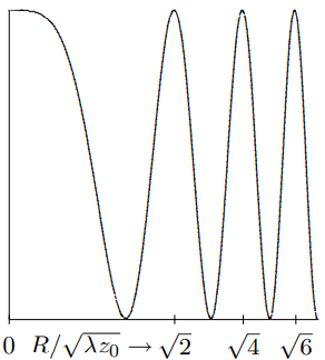
Figure 13.35:The intensity distribution.
If the plate is developed and illuminated by a plane wave, the original spherical wave is reproduced along with another spherical wave moving inward toward a point on the axis a distance beyond the plate, as shown in Figure 13.36. This wave is the real image of Figure 13.33. When a plane wave (dotted lines) illuminates the photographic plate produced in Figure 13.34, diverging (dotted lines) and converging (solid lines) spherical waves are produced.
Zone Plates
The hologram of Figure 13.34 can be used to bring part of plane wave to a focus. The converging spherical wave shown in Figure 13.36 is much stronger than the rest of the wave disturbance at the focus, , , because the amplitude of this part of the wave
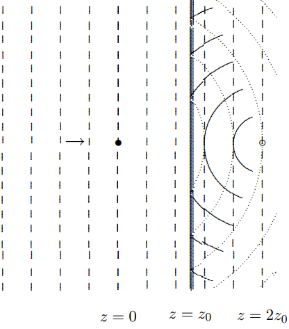
Figure 13.36:A plane wave illuminating the photographic plate.
increases as it approaches the focus. It has the form
where
The same effect can be produced with a cartoon version of the photographic plate made by taking a transparent plate and blacking out the zones for negative in (13.138) where the intensity distribution is less than half the maximum. For example, the first negative zone is the region . The second is the region , etc. The result is a “zone plate.” An example, produced by blacking out the first 4 negative zones is shown in Figure 13.37. These things are quite useful, because they can be easily produced and tailored to any wavelength.
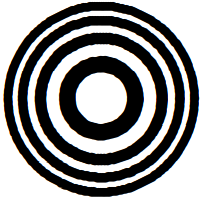
Figure 13.37:A zone plate.
13.10: 13-8- Holography
Nothing prevents us from doing the analysis of a diffraction pattern from a more complicated function, , than that discussed in 13.16. A hologram is just such a diffraction pattern. One of the simplest versions of a hologram is one in which an object is illuminated by a laser, that provides essentially a plane wave. The reflected light, and a part of the laser beam (extracted by some beam splitting technique) are incident on a photographic plate at slightly different angles, as shown schematically in Figure 13.31. The wave incident on the photographic plate has the form
where
13.127 describes the two coherent parts of the light wave incident on the photographic plate. For simplicity, we will assume that the signal in which we are actually interested, the reflected wave with Fourier transform , is small compared to the reference wave . This signal is what we would see if the photographic plate were removed and we placed
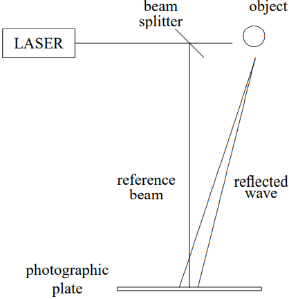
Figure 13.31:Making a hologram.
our eyes in the path of the reflected wave, but out of the path of the laser beam, as shown in Figure 13.32.
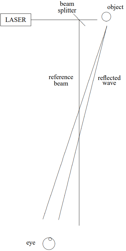
Figure 13.32:Viewing the object.
The photographic plate (we’ll assume it’s at = 0) records only the intensity of the total wave, proportional to
We will drop the terms of order , assuming that is small, although we will be able to see later that they will not actually not make any difference even if is large. If we now make a positive slide from the plate and shine through it a laser beam with the same frequency, , the wave “gets through” where the light intensity on the plate was large and is absorbed where the intensity was small. Thus we have a forced oscillation problem of exactly the sort that we discussed above, with 13.129 playing the role of . The solution for (from 13.19-13.24) is
where c.c. is the complex conjugate wave obtained by taking the complex conjugate of the signal and changing the sign of the dependence to get a wave traveling in the direction. The important thing to note about the complex conjugate wave is that it represents a beam traveling in a different direction from either the signal or the reference beam, because the complex conjugation has changed the sign of and .
The resulting system is shown schematically in Figure 13.33. Your eye sees a reconstructed version of the reflected wave that you would have seen without the photographic plate, as in 13.32. Note that neither the reference beam nor the complex conjugate beam get in the way of your viewing, because they go off at slightly different angles. This is a hologram. Because it is not a picture but a reconstruction of the actual wave that you would have seen in 13.32, it has the surprising property of three-dimensionality that makes a hologram striking.
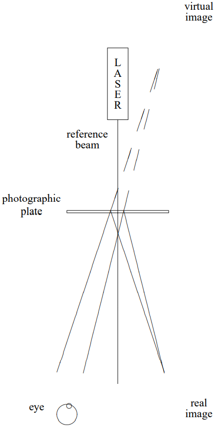
Figure 13.33:Viewing the holographic image.
One might wonder why we choose the angle between the reference beam and the signal to be small. A large angle would have the advantage of getting the reference beam farther out of the way, but it would have an important disadvantage. Consider the intensity pattern on the photographic plate that records the hologram. It is an oscillating pattern with a typical wave number given by the typical value of or . These are of order , where is the angle between the reference beam and the signal. But the distance between neighboring maxima on the photographic plate is therefore of order
where is the wavelength of the light. Since is a very small distance, it pays to pick small to spread out the pattern on the photographic plate.
Note, also, that the order terms that we dropped really don’t do any harm even if is not small. Because their and dependence is proportional to that of the signal times its complex conjugate, the typical and for these terms is zero and they travel roughly in the direction of the reference beam. They don’t reach your eye in 13.33.
For example, see Hecht, chapter 10.
See the discussion starting on page 314.
See, however, the discussion on page 383.
Note that is well-defined () at .
Here we are assuming small angles, so that . In our discussion of diffraction gratings below, we will see what happens when the difference in important.
“Narrow” here means narrow compared to the wavelength of the light — see the moral above.