Although the wave phenomena we can see in the laboratory live in finite regions of space, it is often convenient to analyze them as if the traveling waves come in from and go out to infinity. We have described traveling waves in infinite translation invariant systems. But traveling waves are more complicated and more interesting in systems in which there are boundaries that break the translation symmetry.
Consider the forced oscillation problem in a semiinfinite stretched string that runs from x=0 to x=∞. Suppose that
ψ(0,t)=Acosωt(9.1)
Then what is ψ(x,t)? This is not a well-posed problem, because we only have a boundary condition on one side. Furthermore, ψ(∞,t) does not have a definite value. We can only talk about the value of a function at infinity if the function goes to a constant value. Here, we expect ψ(x,t) to continue to oscillate as x→∞, so we cannot specify it. Instead, we can specify either the incoming (traveling toward the boundary at x=0 in the −x direction) or the outgoing (traveling away from x=0 in the +x direction) traveling waves in the system. This is called a “boundary condition at ∞.”
For example, we could take our boundary condition at infinity to be that no incoming traveling waves appear on the string. Physically, this corresponds to the situtation in which the motion of the string at x=0 is producing the waves. In general, we can write a solution with angular frequency ω as a sum of four real traveling waves
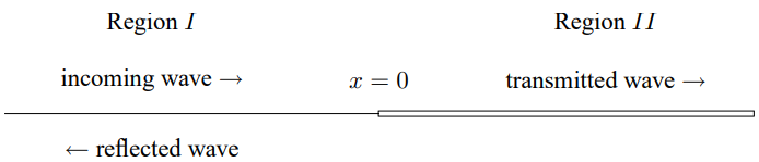
Now consider two semi-infinite strings with the same tension but different densities that are tied together at x=0, as shown in Figure 9.1. Suppose that in the x≤0 region (Region I), there is an incoming traveling wave with amplitude A and angular frequency ω, and in the x≥0 region (Region II), there is no incoming traveling wave. This describes a physical situation in which the incoming wave in I is scattered by the boundary so that the other waves are a transmitted wave in II and a reflected wave in I, both outgoing.
Figure 9.1:Two semi-infinite strings tied together at x=0.
The key to this problem is to think of it as a forced oscillation problem. The incoming traveling wave in region I is what is “causing” all the oscillations. We have put the word in quotes, because the harmonic form, e−iωt, for the oscillation implies that it has been going on forever, so that a philosopher might question this use of cause and effect. Nevertheless, it will help us to think of it this way. If the reflected and transmitted waves are produced by the incoming wave, their amplitudes will also be proportional to e−iωt. As in a conventional forced oscillation problem, we could add on any free oscillations of the system. However, if there is any friction at all, these will die away with time, and we will be left only with the oscillation produced by the incoming traveling wave, proportional to e−iωt. The important thing is that the frequency is the same in both regions, because as in a forced oscillation problem, the frequency is imposed on the system by an external agency, in this case, whatever produced the incoming traveling wave.
In our complex exponential notation in which everything has the irreducible time dependence, e−iωt. Right moving waves are ∝eikxe−iωt and left moving waves are ∝e−ikxe−iωt. In this case, the boundary conditions at ±∞ require that
ψ(x,t)=eikxAe−iωt+RAe−ikxe−iωt(9.6)
for x≤0 in Region I, and
ψ(x,t)=τAeik′xe−iωt(9.7)
for x≥0 in Region II. The k and k′ are
k=ωρI/T,k′=ωρII/T,(9.8)
and R and τ are (in general) complex numbers that determine the reflected and transmitted waves. They are sometimes called the “reflection coefficient” and “transmission coefficient,” or the “amplitudes” for transmission and reflection. Notice that we have defined the reflection and transmission coefficients by taking out a factor of the amplitude, A, of the incoming wave. The amplitude, A, then drops out of all the boundary conditions, and the dimensionless coefficients R and τ are independent of A. This must be so because of the linearity of the system. We know that once we have found the solution, ψ(x,t), for an incoming amplitude, A, we can find the solution for an incoming amplitude, B, by multiplying our solution by B/A. We will keep the parameter, A, in our expressions for ψ(x,t), mostly in order to keep the units right. A has units of length in this example, but in general, the amplitude of the incoming wave will have units of generalized displacement (as in 1.107 and 1.108).
To determine R and τ, we need a boundary condition at x=0 where 9.6 and 9.7 meet. Clearly ψ(x,t) must be continuous at x=0, thus
1+R=τ.(9.9)
We have canceled the common factor of Ae−iωt from both sides. The x derivative must also be continuous (for a massless knot) because the vertical forces on the knot must balance, thus
Note that we could replace the string in Region II by a dashpot with the same impedance, ZII. This must be true because of the local nature of the interactions. The only thing that the string for x<0 knows about the string for x>0 is that it exerts a force at x=0 equal to
−ZII∂t∂ψ(0,t).(9.12)
Thus we also learned what happens when an incoming wave encounters a dashpot with the wrong impedance. The amplitude of the reflected wave is given by R in 9.11.
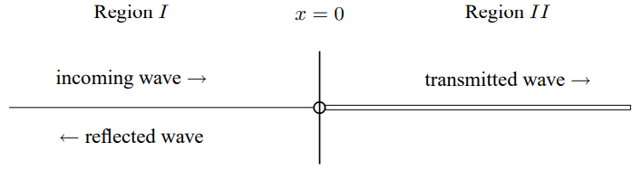
The reflected wave in 9.11 vanishes if k=k′. If k=k′, then ρI=ρII (from 9.8), and the impedance in region I is the same as the impedance in region II. This is a simple example of the important principle of “impedance matching.” There is no reflection if the impedance of the system in region II is the same as the impedance of the system in region I. The argument is the same as for the dashpot in the previous paragraph. What matters in the computation of the reflection coefficient are the forces that act on the string at x=0. Those forces are determined by the impedances in the two regions. Nothing else matters. Consider, for example, the system shown in Figure 9.2 of two semi-infinite strings connected at x=0 to a massless ring which is free to slide in the vertical direction on a frictionless rod. The rod can exert a horizontal force on the ring, so the tensions in the two strings need not be the same. In such a system, we can change both the density and the tension in the string from region I to region II. There will be no reflection so long as the product of the linear mass density and the tension (and thus the impedance, from 8.22) is the same in both regions,
ZI=ρITI=ρIITII=ZII.(9.13)
Figure 9.2:A system in which impedances can be matched.
It is instructive to solve the scattering problem completely for the more general case shown in Figure 9.2. This will give us a feeling for the meaning of impedance. The form of the solution, 9.6 and 9.7 is unchanged, but now the angular wave numbers satisfy
k=ωρI/TI,k′=ωρII/TII.(9.14)
The boundary condition at x=0 arising from the continuity of the string, 9.9, remains unchanged. However, 9.10 arose from the fact that the forces on the massless knot must sum to zero so the acceleration is not infinite. In this case, from 8.21, the contribution of each component of the wave to the total force is proportional to plus or minus the impedance in the relevant region depending on whether it is moving in the +x or the −x direction. Thus the boundary condition is
ZI(1−R)=ZIIτ.(9.15)
Then the reflection and transmission coefficients are
τ=ZI+ZII2ZI,R=ZI+ZIIZI−ZII.(9.16)
We have already discussed the case where the impedances match and the reflection coefficient vanishes. It is also interesting to look at the limits in which R=±1. First consider the limit in which the impedance in region II goes to infinity,
ZII→∞limR=−1.(9.17)
This is situation in which it takes an infinite force to produce a wave in region II. Thus the string in region II does not move at all, and in particular, the point x=0 might as well be a fixed end. The solution, 9.17 ensures that the string does not move at x=0, and therefore that the solution in region I is ψ(x,t)∝sinkx. This solution is an infinite standing wave with a fixed end boundary condition.
In the opposite limit, in which the impedance in region II is zero, we get
ZII→0limR=1.(9.18)
This time, it takes no force at all to produce a wave in region II. Thus the end of region I at x=0 feels no transverse force. It acts like a free end. The solution, 9.18 ensures that ψ(x,t)∝coskx in region I, so the slope of the string vanishes at x=0. This solution is an infinite standing wave with a free end boundary condition.
In this section, we discuss what the displacement in Region I looks like. We will find a useful diagnostic for the presence of reflection. We will also conclude that standing waves are very special.
Look at a wave of the form
Acos(kx−ωt)+RAcos(kx+ωt).(9.19)
This describes an incoming traveling wave with some reflected wave of amplitude R (we could put in an arbitrary phase for the reflected wave but it would complicate the algebra without changing the physics).
For R=±1, this is a standing wave. For R=0, it is a traveling wave. To see how the system interpolates between these two extremes, consider the motion of the crest of the wave, a maximum of 9.19.
To find the maximum, we differentiate with respect to x and set the result to zero. Eliminating the irrelevant factor of A, we get
sin(kx−ωt)+Rsin(kx+ωt)=0,(9.20)
or
(1+R)sinkxcosωt=(1−R)coskxsinωt,(9.21)
or
tankx=1+R1−Rtanωt.(9.22)
9.22 describes (implicitly — we could solve for x as a function of t if we felt like it) the motion of the maximum as a function of time. We can differentiate it to get the velocity:
k(1+tan2kx)∂t∂x=1+R1−Rcos2ωtω.(9.23)
We have left (1+tan2kx) in 9.23 so that we can eliminate it by using 9.22. Thus
where v=ω/k is the phase velocity. When sinωt vanishes, the speed of the maximum is smaller than the phase velocity by a factor of
1+R1−R,(9.25)
while when cosωt vanishes, the speed is larger than the v by the inverse factor,
1−R1+R.(9.26)
The wave thus appears to move in fits and starts. You can easily see this effect if you stare at a system with a lot of reflection. The effect is illustrated in program 9-1.
We can draw a more general moral from this discussion. The general case of wave motion is much more like a traveling wave than like a standing wave. Generically, except for R=±1, the wave crests move with time. As we approach R=±1, one of the two velocities in 9.25 and 9.26 goes to zero and the other goes to infinity. What happens when you are close to R=±1 is then that the wave stays nearly still most of the time, and then moves very quickly to the next nearly stationary position. A standing wave is thus a degenerate special case of a traveling wave in which this motion is unobservable because, in a sense, it is infinitely fast.
It is instructive to consider the power required to produce a traveling wave that is partially reflected. That is, we consider the power required by a transverse force acting at x=0 to produce a wave in the region x>0 that is a linear combination of an outgoing wave moving in the +x direction and an incoming wave moving in the −x direction, such as might be produced by a reflection at some large value of x. Let us imagine the most general one-dimensional case, in a medium with impedance Z:
Now because 9.27 involves waves traveling both in the +x and in the −x direction, we cannot find the force required to produce the wave at the point x by simply multiplying 9.28 by the impedance, Z. However, we can use linearity. We can write ψ(x,t)=ψ+(x,t)+ψ−(x,t), where ψ±(x,t) is the wave moving in the ±x direction. Then from 8.21, the force required to produce ψ+ is
The result, 9.32, has an obvious and important physical interpretation. Positive power is required to produce the outgoing traveling wave, while the incoming wave gives energy back to the system, and thus requires negative power. The power required to produce a general traveling wave is thus proportional to the difference of the squares of the absolute values of the amplitudes of the outgoing and incoming waves.
Note also that we can apply this discussion to the example of reflection at a boundary, discussed above. We can check that energy is conserved in this scattering. The average power required to produce the wave in region I is, from 9.33
ZIω2−ZIω2R2.(9.34)
The average power required to produce the wave in region II is,
Consider the transmission and reflection of waves from a mass, m, at x=0 on a string with linear mass density ρ and tension T, stretched from x=−∞ to x=∞, shown in Figure 9.3. Before we calculate the coefficients for reflection and transmission, let us guess the result in two extreme limits.
msmall – Here we expect that the reflection to be small and the transmission close to one, because in the limit
m→0⇒τ→1 and R→0.(9.36)
mlarge – Here we expect the transmission to be small and the reflection close to −1, because in the limit
m→∞→τ→0 and R→−1.(9.37)
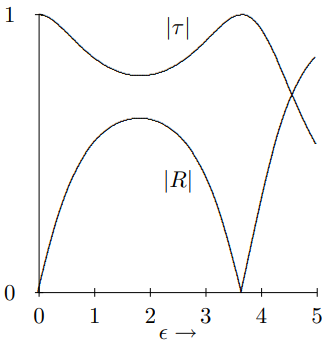
“Large or small compared to what?” you ask! That we can answer by dimensional analysis. The relevant dimensional parameters are m, ω, k, ρ and T. However, one of these is not independent, because of the dispersion relation, 6.5. If we use 6.5 to eliminate T, then ω cannot be relevant to the question, because it is the only thing left that involves the unit of time. The only dimensionless quantity we can build is
ϵ=ρmk=kTmω2.(9.38)
Now that we have guessed, we can do the calculation. It follows from translation invariance and the boundary condition at x=∞ that
ψ(x,t)=Aeikxe−iωt+RAe−ikxe−iωt for x≤0(9.39)
ψ(x,t)=τAeikxe−iωt for x≥0(9.40)
where, as usual, R and τ are “amplitudes” for the reflected and transmitted waves. The boundary conditions are
continuity – The fact that the string doesn’t break implies that it is continuous, so that ψ(0,t) can be computed with either 9.39 or 9.40. This implies
1+R=τ.(9.41)
F=ma– The horizontal component of the tension in the string must be equal on the two sides. Both are about equal to T, for small displacements. However, if there is a kink in the string, the vertical components do not match, as shown in Figure 9.4 (see also 8.16-8.17). The force on the mass is then the tension times the slope for x≥0 minus the tension times the slope for x≤0, thus F=ma becomes
Note that these amplitudes, unlike those in 9.11, are complex numbers. The transmitted and reflected waves do not have the same phase as the incoming wave at the boundary. The phase difference between the transmitted (or reflected) wave is called a “phase shift.” One interesting feature of the solution, 9.45, that we did not guess is that for large ϵ, the small transmitted wave is 90∘ out of phase with the incoming wave.
This scattering is animated in program 9-2. The solution is also decomposed into incoming, transmitted and reflected waves. Stare at the mass and see if you can understand how the kink in the string is related to its acceleration. You can also make the mass larger and smaller to approach the limits 9.36 and 9.37.
Matter is composed of electric charges. This is something of a miracle. We cannot understand it without quantum mechanics. In a purely classical world, there would be no stable atoms or molecules. Because of quantum mechanics, the world does not collapse and we can build stable chunks of matter composed of equal numbers of positive and negative charges. In a chunk of matter in equilibrium, the charge and current are very close to zero when averaged over any large smooth region. However, in the presence of external electric and magnetic fields, such as those produced by an electromagnetic wave, the charges out of which the matter is built can move. This gives rise to what are called “bound” charges and currents, distinguishable from the “free” charges that are not part of the matter itself. These bound charges and currents affect the relation between electric and magnetic fields. In a homogeneous and isotropic material, which is a fancy way of describing a material that does not have any preferred axis, the effects of the matter (averaged over large regions) can be incorporated by replacing the constants ϵ0 and μ0 by the permittivity and permeability, ϵ and μ. Then Maxwell’s equations for electromagnetic waves, 8.35-8.37, are modified to1
is called the index of refraction of the material. 1/n is the ratio of the speed of light in the material to the speed of light in vacuum. In terms of n, we can write 9.52 as
βy±=±cnεx±,βx±=∓cnεy±.(9.54)
Note also that we can rewrite 9.50 in the following useful form:
k=ncω.(9.55)
For fixed frequency, the wave number is proportional to the index of refraction. For most transparent materials, μ is very close to 1, and can be ignored. But ϵ can be very different from 1, and is often quite important. For example, the index of refraction of ordinary glass is about 1.5 (it varies slightly with frequency, but we will discuss the interesting and familiar consequences of this later, when we treat waves in three dimensions).
Let us now consider a plane wave in the +z direction in a universe that is filled with a dielectric material with index of refraction n=ϵ/ϵ0, for z<0 and filled with another dielectric material with index of refraction n′=ϵ′/ϵ0, for z>0. The boundary between the two dielectrics, the plane z=0, is analogous to the boundary between two regions of the rope in Figure 9.1. We would, therefore, expect some reflection from this surface.
Because the electric field in a plane electromagnetic wave is perpendicular to its direction of motion, we know that in this case that it is in the x-y plane. It doesn’t matter in what direction the electric field of our incoming plane wave is pointing in the x-y plane. That is clear by symmetry. The system looks the same if we rotate it around the z axis, thus we can always rotate until our e+ vector is pointing in some convenient direction, say the x direction. It is then pretty obvious that the reflected and transmitted waves will also have their electric fields in the ±x direction. Actually, we can turn this into a symmetry argument too. If we reflect the system in the x-z plane, both the incoming wave and the dielectric are unchanged, but any y component of the transmitted or reflected waves would change sign. Thus these components must vanish, by symmetry. Magnetic fields work the other way, because of the cross product of vectors in their definition. Thus we can write
Ex(z,t)=Aei(kz−ωt)+RAei(−kz−ωt)By(z,t)=cnAei(kz−ωt)−cnRAei(−kz−ωt) for z<0,(9.56)
and
Ex(z,t)=τAei(kz−ωt)By(z,t)=cn′τAei(kz−ωt) for z>0,(9.57)
where we have continued our convention of calling the amplitude of the incoming wave A. Here, A has units of electric field. In 9.56 and 9.57, we have used 9.54 to get the B field from the E field.
To compute R and τ, we need the boundary conditions at z=0. For this we go back to Maxwell. The only way to get a discontinuity in the electric field is to have a sheet of charge. In a dielectric, charge builds up on the boundary only if there is a polarization perpendicular to the boundary. In this case, the electric fields, and therefore the polarizations, are parallel to the boundary, and thus the E field is continuous at z=0. The only way to get a discontinuity of the magnetic field, B, is to have a sheet of current. If μ were not equal to 1 in one of the materials, then we would have a nonzero magnetization, and we would have to worry about current sheets at the boundary. However, because these are only dielectrics, and μ=1 in both, there is no magnetization and the B field is continuous at z=0 as well. Thus we can immediately read off the boundary conditions:
1+R=τ,n(1−R)=n′τ.(9.58)
Because of 9.55, the boundary condition 9.58 is equivalent to
1+R=τ,k(1−R)=k′τ,(9.59)
which looks exactly like 9.9 and 9.10. We can simply take over the results of 9.11,
Next consider the reflection and transmission from two masses on a string, as in Figure 9.5. Now translation invariance and the boundary condition at x=∞ imply that
ψ(x,t)=TIAeikxe−iωt+RIAe−ikxe−iωt for 0≤x≤L,(9.62)
ψ(x,t)=τAeikxe−iωt for x≥L.(9.63)
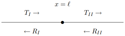
Figure 9.6:The general scattering problem from a mass on a string.
We could solve this problem in the same way, simply imposing boundary conditions twice, at x=0 and at x=L, but there is a systematic way of doing this that is very useful. Consider first the general scattering problem from a single mass at x=ℓ, with both incoming and outgoing waves on both sides, as shown in Figure 9.6. This is the most general possible thing that can happen in scattering from a single mass, and we will be able to use the result to do much more complicated problems without any additional work. The general solution has the form
ψ(x,t)=TIAeikxe−iωt+RIAe−ikxe−iωt for x≤ℓ,(9.64)
ψ(x,t)=TIIAeikxe−iωt+RIIAe−ikxe−iωt for x≥ℓ.(9.65)
The important point is that because of linearity, the result 9.69 can be written in matrix form:
(TIRI)=d(ℓ)(TIIRII)(9.70)
where the matrix d(ℓ)
d(ℓ)=21((2−iϵ)iϵe2ikℓ−iϵe−2ikℓ(2+iϵ)).(9.71)
The matrix, d(ℓ), is a “transfer matrix.” It allows us to get from the amplitudes in one region to those in the next by just doing a matrix multiplication. We can use this to solve the two mass problem without any further calculation except a matrix multiplication. Comparing the general result, 9.70, with the two mass problem, Figure 9.5, we see immediately that
Figure 9.8:The general scattering problem for a change of k.
Let us return to the simple example at the beginning of the chapter of a boundary between two regions of string with different values of k. This is a very important example because its general features are characteristic of many important physical systems. For example, when a light-wave encounters a transparent medium, the k value changes. That situation is somewhat more complicated because of the three-dimensional nature of light waves and because of polarization. However the analogy between 9.59 and 9.9 and 9.10 means that we can take over the discussion of of the string directly to electromagnetic waves reflecting from a dielectric boundary perpendicular to the direction of the wave. In this section, we apply the general method of transfer matrices discussed in the previous section to this important example. Thus we consider the situation shown in Figure 9.8. where the waves have the form
ψ(x,t)=Ae−iωt(TIeik1x+RIe−ik1x) in I,(9.78)
ψ(x,t)=Ae−iωt(TIIeik2x+RIIe−ik2x) in II.(9.79)
Then as in 9.9 and 9.10, the boundary conditions are that ψ is continuous at x=ℓ, which implies
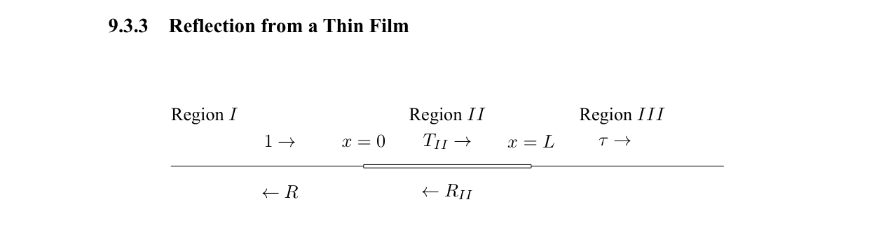
Consider the situation shown in Figure 9.9. where the wave numbers are k1 for x≤0, k2 for 0≤x≤L and k3 for x≥L. As usual, translation invariance plus the boundary condition at infinity (that the incoming wave in I has amplitude, A, and that there is only an outgoing wave in III) implies
ψ(x,t)=Ae−iωt(eik1x+Re−ik1x) for x≤0ψ(x,t)=Ae−iωt(TIIeik2x+RIIe−ik2x) for 0≤x≤L,ψ(x,t)=τAe−iωteik3x for L≤x.(9.89)
Then we know from the results of the previous section that
Often we are interested in the situation k3=k1, that describes a film (in one-dimension, a film is just a region in x) in an otherwise homogeneous medium. This is then a one-dimensional analog of the reflection of light from a soap bubble. Then the transfer matrix looks like
Here we see the phenomenon of resonant transmission. The wave does not get reflected at all if the thickness of the film is an integral or half-integral number of wavelengths. Note, also, that when k2→k1, τ→1 and R→0 as they should, because in this limit there is no boundary.
The reflection in 9.98 varies rapidly with k2, as shown Figure 9.10, where we plot the intensity of the reflected wave versus k2 for fixed ratio k1/k2=3. It is this rapid variation of the intensity of reflected light as a function of wavelength that is responsible for the familiar color patterns on thin films like soap bubbles and oil slicks.
Figure 9.10:Graph of ∣R∣2 versus k2 for k1/k2=3.
We will not work out the general case of k1=k3, simply because the algebra is a mess. However, one important special case is worth noting. Suppose that you have a boundary between media in which the wave number of your traveling wave are k1 and k3. Normally, you find reflection at the boundary. The question is, can you add an intermediate film layer with wave number k2, that eliminates all reflection? The answer is yes. First you must adjust the wave number in the film to be the geometric mean of k1 and k3, so that
It is easy to check that the reflection vanishes when there are a half-odd-integral number of wavelengths in the intermediate region,
k2L=(2n+1)2π.(9.100)
In qualitative terms, the reflection vanishes because of a destructive interference between the reflected waves from the two boundaries. This has practical applications to nonreflective coatings for optical components.
 9-2
9-2