The climax of this book comes early. Here we identify the crucial features of a system that supports waves — space translation invariance and local interactions.
5.1: Space Translation Invariance
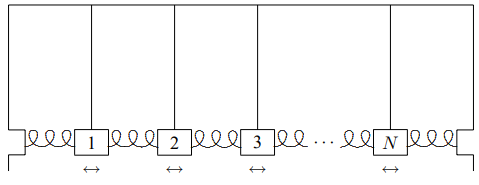
Figure 5.1:A finite system of coupled pendulums.
The typical system of coupled oscillators that supports waves is one like the system of identical coupled pendulums shown in Figure 5.1. This system is a generalization of the system of two coupled pendulums that we studied in chapters 3 and 4. Suppose that each pendulum bob has mass , each pendulum has length , each spring has spring constant and the equilibrium separation between bobs is . Suppose further that there is no friction and that the pendulums are constrained to oscillate only in the direction in which the springs are stretched. We are interested in the free oscillation of this system, with no external force. Such an oscillation, when the motion is parallel to the direction in which the system is stretched in space is called a “longitudinal oscillation”. Call the longitudinal displacement of the th bob from equilibrium . We can organize the displacements into a vector, (for reasons that will become clear below, it would be confusing to use , so we choose a different letter, the Greek letter psi, which looks like in lower case and when capitalized):
Then the equations of motion (for small longitudinal oscillations) are
where is the diagonal matrix with ’s along the diagonal,
and has diagonal elements , next-to-diagonal elements , and zeroes elsewhere,
The in the next-to-diagonal elements has exactly the same origin as the in the matrix in 3.78. It describes the coupling of two neighboring blocks by the spring. The on the diagonal is analogous to the on the diagonal of 3.78. The difference in the factor of 2 in the coefficient of arises because there are two springs, one on each side, that contribute to the restoring force on each block in the system shown in Figure 5.1, while there was only one in the system shown in Figure 3.1. Thus has the form
where
It is interesting to compare the matrix, 5.5, with the matrix, 4.43, from the previous chapter. In both cases, the diagonal elements are all equal, because of the symmetry. The same goes for the next-to-diagonal elements. However, in 5.5, all the rest of the elements are zero because the interactions are only between nearest neighbor blocks. We call such interactions “local.” In 4.43, on the other hand, each of the masses interacts with all the others. We will use the local nature of the interactions below.
We could try to find normal modes of this system directly by finding the eigenvectors of , but there is a much easier and more generally useful technique. We can divide the physics of the system into two parts, the physics of the coupled pendulums, and the physics of the walls. To do this, we first consider an infinite system with no walls at all.
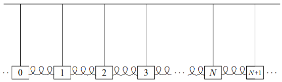
Figure 5.2:A piece of an infinite system of coupled pendulums.
Notice that in Figure 5.2, we have not changed the interior of the system shown in Figure 5.1 at all. We have just replaced the walls by a continuation of the interior.
Now we can find all the modes of the infinite system of Figure 5.2 very easily, making use of a symmetry argument. The infinite system of Figure 5.2 looks the same if it is translated, moved to the left or the right by a multiple of the equilibrium separation, . It has the property of “space translation invariance.” Space translation invariance is the symmetry of the infinite system under translations by multiples of . In this example, because of the discrete blocks and finite length of the springs, the space translation invariance is “discrete.” Only translation by integral multiples of give the same physics. Later, we will discuss continuous systems that have continuous space translation invariance. However, we will see that such systems can be analyzed using the same techniques that we introduce in this chapter.
We can use the symmetry of space translation invariance, just as we used the reflection and rotation symmetries discussed in the previous chapter, to find the normal modes of the infinite system. The discrete space translation invariance of the infinite system (the symmetry under translations by multiples of ) allows us to find the normal modes of the infinite system in a simple way.
Most of the modes that we find using the space translation invariance of the infinite system of Figure 5.2 will have nothing to do with the finite system shown in Figure 5.1. But if we can find linear combinations of the normal modes of the infinite system of Figure 5.2 in which the 0th and + 1st blocks stay fixed, then they must be solutions to the equations of motion of the system shown in Figure 5.1. The reason is that the interactions between the blocks are “local” — they occur only between nearest neighbor blocks. Thus block 1 knows what block 0 is doing, but not what block −1 is doing. If block 0 is stationary it might as well be a wall because the blocks on the other side do not affect block 1 (or any of the blocks 1 to ) in any way. The local nature of the interaction allows us to put in the physics of the walls as a boundary condition after solving the infinite problem. This same trick will also enable us to solve many other problems.
Let us see how it works for the system shown in Figure 5.1. First, we use the symmetry under translations to find the normal modes of the infinite system of Figure 5.2. As in the previous two chapters, we describe the solutions in terms of a vector, . But now has an infinite number of components, where the integer runs from to . It is a little inconvenient to write this infinite vector down, but we can represent a piece of it:
Likewise, the matrix for the system is an infinite matrix, not easily written down, but any piece of it (along the diagonal) looks like the interior of 5.5:
This system is “space translation invariant” because it looks the same if it is moved to the left a distance . This moves block to where block used to be, thus if there is a mode with components , there must be another mode with the same frequency, represented by a vector, , with components
The symmetry matrix, , is an infinite matrix with 1s along the next-to-diagonal. These are analogous to the 1s along the next-to-diagonal in 4.40. Now, however, the transformation never closes on itself. There is no analog of the 1 in the lower left-hand corner of 4.40, because the infinite matrix has no corner. We want to find the eigenvalues and eigenvectors of the matrix , satisfying
or equivalently (from 5.9), the modes in which and are proportional:
where is some nonzero constant.[1]
Equation 5.11 can be solved as follows: Choose . Then , , etc., so that for all nonnegative . We can also rewrite 5.11 as , so that , , etc. Thus the solution is
Now that we know the form of the normal modes, it is easy to get the corresponding frequencies by acting on 5.12 with the matrix, 5.8. This gives
or inserting 5.13,
This is true for all , which shows that 5.13 is indeed an eigenvector (we already knew this from the symmetry argument, 4.22, but it is nice to check when possible), and the eigenvalue is
Notice that for almost every value of , there are two normal modes, because we can interchange and without changing 5.16. The only exceptions are
corresponding to . The fact that there are at most two normal modes for each value of will have a dramatic consequence. It means that we only have to deal with two normal modes at a time to implement the physics of the boundary. This is a special feature of the one-dimensional system that is not shared by two- and three-dimensional systems. As we will see, it makes the one-dimensional system very easy to handle.
Boundary Conditions
 5-1
5-1
We have now solved the problem of the oscillation of the infinite system. Armed with this result, we can put back in the physics of the walls. Any (except ) gives a pair of normal modes for the infinite system of Figure 5.2. But only special values of will work for the finite system shown in Figure 5.1. To find the normal modes of the system shown in Figure 5.1, we use (4.56), the fact that any linear combination of the two normal modes with the same angular frequency, , is also a normal mode. If we can find a linear combination that vanishes for and for , it will be a normal mode of the system shown in Figure 5.1. It is the vanishing of the normal mode at and that are the “boundary conditions” for this particular finite system.
Let us begin by trying to satisfy the boundary condition at . For each possible value of , we have to worry about only two normal modes, the two solutions of 5.16 for . So long as , we can find a combination that vanishes at ; just subtract the two modes and to get a vector
or in components
The first thing to notice about 5.19 is that cannot vanish for any unless . Thus if we are to have any chance of satisfying the boundary condition at , we must assume that
Then from 5.19,
Now we can satisfy the boundary condition at by setting . This implies , or
Thus the normal modes of the system shown in Figure 5.1 are
Other values of do not lead to new modes, they just repeat the modes already shown in 5.23. The corresponding frequencies are obtained by putting 5.20-5.21 into 5.16, to get
From here on, the analysis of the motion of the system is the same as for any other system of coupled oscillators. As discussed in chapter 3, we can take a general motion apart and express it as a sum of the normal modes. This is illustrated for the system of coupled pendulums in program 5-1 on the program disk. The new thing about this system is the way in which we obtained the normal modes, and their peculiarly simple form, in terms of trigonometric functions. We will get more insight into the meaning of these modes in the next section. Meanwhile, note the way in which the simple modes can be combined into the very complicated motion of the full system.
5.2: k and Dispersion Relations
So far, the equilibrium separation between the blocks, , has not appeared in the analysis. Everything we have said so far would be true even if the springs had random lengths, so long as all spring constants were the same. In such a case, the “space translation invariance” that we used to solve the problem would be a purely mathematical device, taking the original system into a different system with the same kind of small oscillations. Usually, however, in physical applications, the space translation invariance is real and all the inter-block distances are the same. Then it is very useful to label the blocks by their equilibrium position. Take to be the position of the left wall (or the 0th block). Then the first block is at , the second at , etc., as shown in Figure 5.3. We can describe the displacement of all the blocks by a function , where is the displacement of the th block (the one with equilibrium position ). Of course, this function is not very well defined because we only care about its values at a discrete set of points. Nevertheless, as we will see below when we discuss the beaded string, it will help us understand what is going on if we draw a smooth curve through these points.
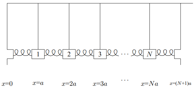
Figure 5.3:The coupled pendulums with blocks labeled by their equilibrium positions.
In the same way, we can describe a normal mode of the system shown in Figure 5.1 (or the infinite system of Figure 5.2) as a function where
In this language, space translation invariance, 5.11, becomes
It is conventional to write the constant as an exponential
Any nonzero complex number can be written as a exponential in this way. In fact, we can change by a multiple of without changing , thus we can choose the real part of to be between and
If we put 5.13 and 5.27 into 5.25, we get
This suggests that we take the function describing the normal mode corresponding to 5.27 to be
The mode is determined by the number satisfying 5.28.
The parameter (when it is real) is called the angular wave number of the mode. It measures the waviness of the normal mode, in radians per unit distance. The “wavelength” of the mode is the smallest length, (the Greek letter lambda), such that a change of by leaves the mode unchanged,
In other words, the wavelength is the length of a complete cycle of the wave, radians. Thus the wavelength, , and the angular wave number, , are inversely related, with a factor of ,
In this language, the normal modes of the system shown in Figure 5.1 are described by the functions
with
where is the total length of the system. The important thing about 5.33 and 5.34 is that they do not depend on the details of the system. They do not even depend on . The normal modes always have the same shape, when the system has length . Of course, as increases, the number of modes increases. For fixed L, this happens because decreases as increases and thus the allowed range of (remember 5.28) increases.
The forms 5.33 for the normal modes of the space translation invariant system are called “standing waves.” We will see in more detail below why the word “wave” is appropriate. The word “standing” refers to the fact that while the waves are changing with time, they do not appear to be moving in the direction, unlike the “traveling waves” that we will discuss in chapter 8 and beyond.
Dispersion Relation
In terms of the angular wave number , the frequency of the mode is (from 5.16 and 5.27)
Such a relation between (actually because is an even function of ) and is called a “dispersion relation” (we will learn later why the name is appropriate). The specific form 5.35 is a characteristic of the particular infinite system of Figure 5.2. It depends on the masses and spring constants and pendulum lengths and separations.
But it does not depend on the boundary conditions. Indeed, we will see below that 5.35 will be useful for boundary conditions very different from those of the system shown in Figure 5.1.
The dispersion relation depends only on the physics of the infinite system.
Indeed, it is only through the dispersion relation that the details of the physics of the infinite system enters the problem. The form of the modes, , is already determined by the general properties of linearity and space translation invariance.
We will call 5.35 the dispersion relation for coupled pendulums. We have given it a special name because we will return to it many times in what follows. The essential physics is that there are two sources of restoring force: gravity, that tends to keep all the masses in equilibrium; and the coupling springs, that tend to keep the separations between the masses fixed, but are unaffected if all the masses are displaced by the same distance. In 5.35, the constants always satisfy , as you see from 5.6.
The limit is especially interesting. This happens when there is no gravity (or ). The dispersion relation is then
Note that the mode with now has zero frequency, because all the masses can be displaced at once with no restoring force.[2]
5.3: Waves
Beaded String

Figure 5.4:The beaded string in equilibrium.
Another instructive system is the beaded string, undergoing transverse oscillations. The oscillations are called “transverse” if the motion is perpendicular to the direction in which the system is stretched. Consider a massless string with tension , to which identical beads of mass are attached at regular intervals, . A portion of such a system in its equilibrium configuration is depicted in Figure 5.4. The beads cannot oscillate longitudinally, because the string would break.[3] However, for small transverse oscillations, the stretching of the string is negligible, and the tension and the horizontal component of the force from the string are approximately constant. The horizontal component of the force on each block from the string on its right is canceled by the horizontal component from the string on the left. The total horizontal force on each block is zero (this must be, because the blocks do not move horizontally). But the strings produces a transverse restoring force when neighboring beads do not have the same transverse displacement, as illustrated in Figure 5.5. The force of the string on bead 1 is shown, along with the transverse component. The dotted lines complete similar triangles, so that . You can see from Figure 5.5 that the restoring force, in the figure, for small transverse oscillations is linear, and corresponds to a spring constant .
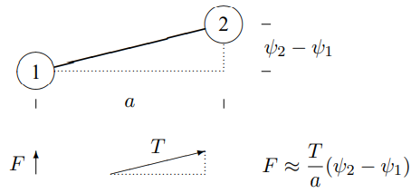
Figure 5.5:Two neighboring beads on a beaded string.
Thus 5.37 is also the dispersion relation for the small transverse oscillations of the beaded string with
where is the string tension, is the bead mass and is the separation between beads. The dispersion relation for the beaded string can thus be written as
This dispersion relation, 5.39, has the interesting property that as . This is discussed from the point of view of symmetry in appendix C, where we discuss the connection of this dispersion relation with what are called “Goldstone bosons.” Here we should discuss the special properties of the mode with exactly zero angular frequency, . This is different from all other angular frequencies because we do not get a different time dependence by complex conjugating the irreducible complex exponential, . But we need two solutions in order to describe the possible initial conditions of the system, because we can specify both a displacement and a velocity for each bead. The resolution of this dilemma is similar to that discussed for critical damping in chapter 2 (see 2.12). If we approach from nonzero , we can form two independent solutions as follows:4
The first, for , describes a situation in which all the beads are sitting at some fixed position. The second describes a situation in which all of the beads are moving together at constant velocity in the transverse direction.
Precisely analogous things can be said about the dependence of the mode. Again, approaching from nonzero , we can form two modes,
The second mode here describes a situation in which each subsequent bead is more displaced. The transverse force on each bead from the string on the left is canceled by the force from the string on the right.
Fixed Ends
 5-2
5-2
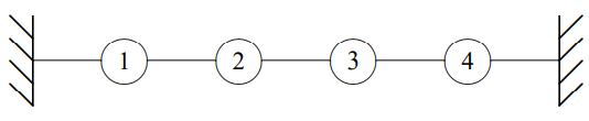
Figure 5.6:A beaded string with fixed ends.
Now suppose that we look at a finite beaded string with its ends fixed at and , as shown in Figure 5.6. The analysis of the normal modes of this system is exactly the same as for the coupled pendulum problem at the beginning of the chapter. Once again, we imagine that the finite system is part of an infinite system with space translation invariance and look for linear combinations of modes such that the beads at and are fixed. Again this leads to 5.33. The only differences are:
the frequencies of the modes are different because the dispersion relation is now given by 5.39;
5.33 describes the transverse displacements of the beads.
This is a very nice example of the standing wave normal modes, 5.33, because you can see the shapes more easily than for longitudinal oscillations. For four beads (), the four independent normal modes are illustrated in , where we have made the coupling strings invisible for clarity. The fixed imaginary beads that play the role of the walls are shown (dashed) at and . Superimposed on the positions of the beads is the continuous function, , for each value, represented by a dotted line. Note that this function does not describe the positions of the coupling strings, which are stretched straight between neighboring beads.
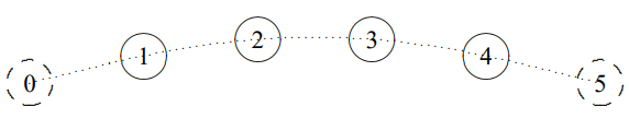
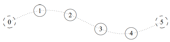
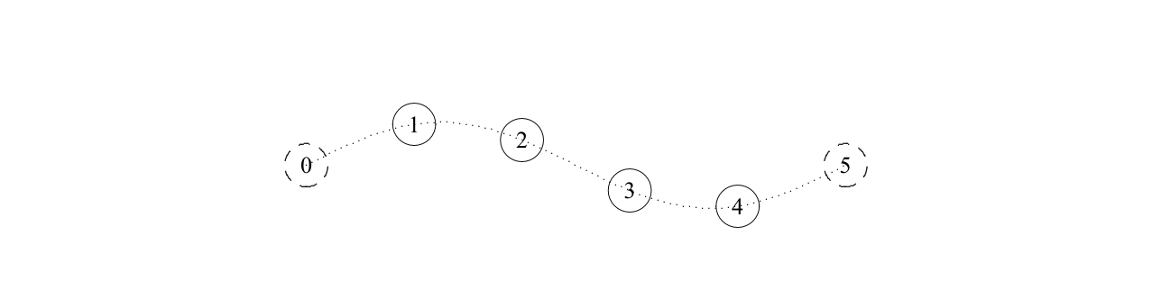
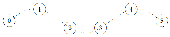
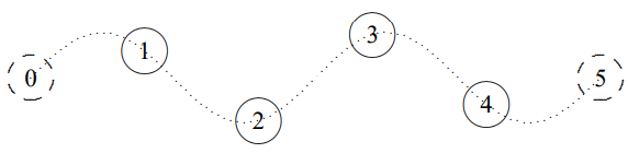
It is pictures like that justify the word “wave” for these standing wave solutions. They are, frankly, wavy, exhibiting the sinusoidal space dependence that is the sine qua non of wave phenomena.
The transverse oscillation of a beaded string with both ends fixed is illustrated in program 5-2, where a general oscillation is shown along with the normal modes out of which it is built. Note the different frequencies of the different normal modes, with the frequency increasing as the modes get more wavy. We will often use the beaded string as an illustrative example because the modes are so easy to visualize.
4You can evaluate the limits easily, using the Taylor series for .
5.4: Free Ends
Let us work out an example of forced oscillation with a different kind of boundary condition. Consider the transverse oscillations of a beaded string. For definiteness, we will take four beads so that this is a system of four coupled oscillators. However, instead of coupling the strings at the ends to fixed walls, we will attach them to massless rings that are free to slide in the transverse direction on frictionless rods. The string then is said to have its ends free (at least for transverse motion). Then the system looks like the diagram in Figure 5.11, where the oscillators move up and down in the plane of the paper: Let us find its normal modes.
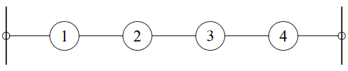
Figure 5.11:A beaded string with free ends.
Normal Modes for Free Ends
 5-3
5-3
As before, we imagine that this is part of an infinite system of beads with space translation invariance. This is shown in Figure 5.12. Here, the massless rings sliding on frictionless rods have been replaced by the imaginary (dashed) beads, 0 and 5. The dispersion relation is just the same as for any other infinite beaded string, 5.39. The question is, then, what kind of boundary condition on the infinite system corresponds to the physical boundary condition, that the end beads are free on one side? The answer is that we must have the first imaginary bead on either side move up and down with the last real bead, so that the coupling string from bead 0 is horizontal and exerts no transverse restoring force on bead 1 and the coupling string from bead 5 is horizontal and exerts no transverse restoring force on bead 4:

Figure 5.12:Satisfying the boundary conditions in the finite system.
We will work in the notation in which the beads are labeled by their equilibrium positions. The normal modes of the infinite system are then . But we haven’t yet had to decide where we will put the origin. How do we form a linear combination of the complex exponential modes, , and choose to be consistent with this boundary condition? Let us begin with 5.42. We can write the linear combination, whatever it is, in the form
Any real linear combination of can be written in this way up to an overall multiplicative constant (see 1.96). Now if
where is the position of the th block, then either
has a maximum or minimum at , or
is a multiple of .
Let us consider case 1. We will see that case 2 does not give any additional modes. We will choose our coordinates so that the point , midway between and , is . We don’t care about the overall normalization, so if the function has a minimum there, we will multiply it by −1, to make it a maximum. Thus in case 1, the function has a maximum at , which implies that we can take . Thus the function is simply . The system with this labeling is shown in Figure 5.13. The displacement of the th bead is then
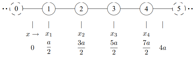
Figure 5.13:The same system of oscillators labeled more cleverly.
It should now be clear how to impose the boundary condition, 5.43, on the other end. We want to have a maximum or minimum midway between bead 4 and bead 5, at . We get a maximum or minimum every time the argument of the cosine is an integral multiple of . The argument of the cosine at is , where is the angular wave number. Thus the boundary condition will be satisfied if the mode has for integer . Then
Thus the modes are
For , the modes just repeat, because .
In 5.48, is the trivial mode in which all the beads move up and down together. This is possible because there is no restoring force at all when all the beads move together. As discussed above (see 5.40) the beads can all move with a constant velocity because for this mode. Note that case 2, above, gives the same mode, and nothing else, because if , then 5.44 has the same value for all . The remaining modes are shown in . This system is illustrated in program 5-3 on the program disk.
![n = 1, A_{j}=\cos [(j-1 / 2) \pi / 4].](/physicsOfWaves/build/lt-33679-clipboard_e-757ee2930e7b23a38d7c18e93353443e.png)
Figure 5.14:, .
![n = 2, A_{j}=\cos [(j-1 / 2) 2 \pi / 4].](/physicsOfWaves/build/lt-33680-clipboard_e-e1b6a953745feabbf15ad0d7ce0eaf3a.png)
Figure 5.15:, .
5.5: Forced Oscillations and Boundary Conditions
Forced oscillations can be analyzed using the methods of chapter 3. This always works, even for a force that acts on each of the parts of the system independently. Very often, however, for a space translation invariant system, we are interested in a different sort of forced oscillation problem, one in which the external force acts only at one end (or both ends). In this case, we can solve the problem in a much simpler way using boundary conditions. An example of this sort is shown in Figure 5.17.
![n = 3, A_{j}=\cos [(j-1 / 2) 3 \pi / 4] ..](/physicsOfWaves/build/lt-33681-clipboard_e-4083de476bcf580e5d18e8635de285b3.png)
Figure 5.16:, .
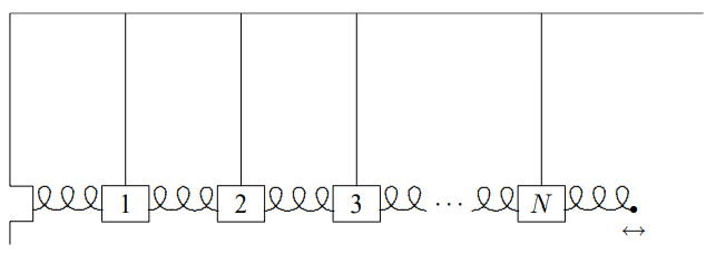
Figure 5.17:A forced oscillation problem in a space translation invariant system.
This is the system of 5.1, except that one wall has been removed and the end of the spring is constrained by some external agency to move back and forth with a displacement
As usual, in a forced oscillation problem, we first consider the driving term, in this case the fixed displacement of the st block, 5.49, to be the real part of a complex exponential driving term,
Then we look for a steady state solution in which the entire system is oscillating with the driving frequency , with the irreducible time dependence, .
If there is damping from a frictional force, no matter how small, this will be the steady state solution that survives after all the free oscillations have decayed away. We can find such solutions by the same sort of trick that we used to find the modes of free oscillation of the system. We look for modes of the infinite system and put them together to satisfy boundary conditions.
This situation is different from the free oscillation problem. In a typical free oscillation problem, the boundary conditions fix . Then we determine from the dispersion relation. In this case, the boundary conditions determine instead. Now we must use the dispersion relation, 5.35, to find the wave number .
Solving 5.35 gives
We must combine the modes of the infinite system, , to satisfy the boundary conditions at and . As for the system 5.1, the condition that the system be stationary at leads to a mode of the form
for some amplitude . But now the condition at determines not the wave number (that is already fixed by the dispersion relation), but the amplitude .
Thus
Notice that if is a normal mode frequency of the system 5.1 with no damping, then 5.54 doesn’t make sense because vanishes. That is as it should be. It corresponds to the infinite amplitude produced by a driving force on resonance with a normal frequency of a frictionless system. In the presence of damping, however, as we will discuss in chapter 8, the wave number is complex because the dispersion relation is complex. We will see later that if is complex, cannot vanish. Even if the damping is very small, of course, we do not get a real infinity in the amplitude as we go to the resonance. Eventually, nonlinear effects take over. Whether it is nonlinearity or the damping that is more important near any given resonance depends on the details of the physical system.[4]
Forced Oscillations with a Free End
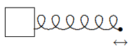
Figure 5.18:Forced oscillation of a mass on a spring.
As another example, we will now discuss again the forced longitudinal oscillations of the simple system of a mass on a spring, shown in Figure 5.18. The physics here is the same as that of the system in Figure 2.9, except that to begin with, we will ignore damping. The block has mass . The spring has spring constant and equilibrium length . To be specific, imagine that this block sits on a nearly frictionless table, and that you are holding onto the other end of the spring, moving it back and forth along the table, parallel to the direction of the spring, with displacement
The question is, how does the block move? We already know how to solve this problem from chapter 2. Now we will do it in a different way, using space translation invariance, local interactions and boundary conditions. It may seem surprising that we can treat this problem using the techniques we have developed to deal with space translation invariant systems, because there is only one block. Nevertheless, that is what we are going to do. Certainly nothing prevents us from extending this system to an infinite system by repeating the block-spring combination. The infinite system then has the dispersion relation of the beaded string (or of the coupled pendulum for ):
The relevant part of the infinite system is shown in Figure 5.19. The point is that we can impose boundary conditions on the infinite system, Figure 5.19, that make it equivalent to Figure 5.18.

Figure 5.19:Part of the infinite system.
We begin by imagining that the displacement is complex, , so that at the end, we will take the real part to recover the real result of 5.55. Thus, we take
Then to ensure that there is no force on block 1 from the imaginary spring on the left, we must take
To satisfy 5.58, we can argue as in Figure 5.13 that
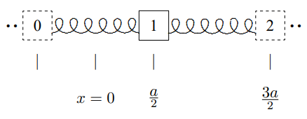
Figure 5.20:A better definition of the zero of .
where is defined as shown in Figure 5.20.
Now since the equilibrium position of block 2 is , we substitute
into 5.57, to obtain
Then the final result is
or in real form
We can now use the dispersion relation. First use trigonometry,
to write
or substituting 5.56,
where is the free oscillation frequency of the system,
This is exactly the same resonance formula that we got in chapter 2.
Generalization
The real advantage of the procedure we used to solve this problem is that it is easy to generalize it. For example, suppose we look at the system shown in Figure 5.21.
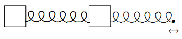
Figure 5.21:A system with two blocks.
Here we can go to the same infinite system and argue that the solution is proportional to where is defined as shown in Figure 5.22. Then the same argument leads to the result for the displacements of blocks 1 and 2:
You should be able to generalize this to arbitrary numbers of blocks.
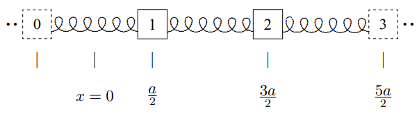
Figure 5.22:The infinite system.
5.6: Coupled LC Circuits
We saw in chapter 1 the analogy between the circuit in Figure 1.10 and a corresponding system of a mass and springs in Figure 1.11. In this section, we discuss what happens when we put circuits together into a space translation invariant system.
For example, consider an infinite space translation invariant circuit, a piece of which is shown in Figure 5.23. One might guess, on the basis of the discussion in chapter 1, that the circuit in Figure 5.23 is analogous to the combination of springs and masses shown in
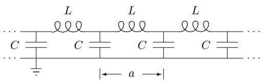
Figure 5.23:A an infinite system of coupled circuits.
Figure 5.24, with the correspondence between the two systems being:
where is the displacement of the th block to the right and is the charge that has been “displaced” through the th inductor from the equilibrium situation with the capacitors uncharged. In fact, this is right, and we could use 5.69 to write down the dispersion relation for the Figure 5.23. However, with our powerful tools of linearity and space translation invariance, we can solve the problem from scratch without too much effort. The strategy will be to write down what we know the solution has to look like, from space translation invariance, and then work backwards to find the dispersion relation.
.](/physicsOfWaves/build/lt-33690-clipboard_e-a850febd667fad5297ca72bd48eea1cb.png)
Figure 5.24:A mechanical system analogous to Figure 5.23.
The starting point should be familiar by now. Because the system is linear and space translation invariant, the modes of the infinite system are proportional to . Therefore all physical quantities in a mode, voltages, charges, currents, whatever, must also be proportional to . In this case the variable, , is really just a label. The electrical properties of the circuit do not depend very much on the disposition of the elements in space.6The dispersion relation will depend only on , where is the separation between the identical parts of the system (see 5.35). However, it is easier to think about the system if it is physically laid out into a space translation invariant configuration, as shown in Figure 5.23.
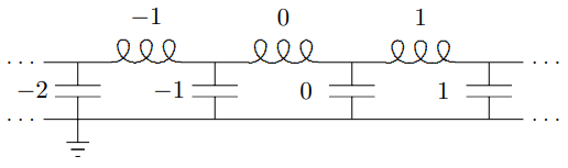
Figure 5.25:A labeling for the infinite system of coupled circuits.
In particular, let us label the inductors and capacitors as shown in Figure 5.25. Then the charge displaced through the th inductor in the mode with angular wave number, , is
for some constant charge, . Note that we could just as well take the time dependence to be , , or . It does not matter for the argument below. What matters is that when we differentiate twice with respect to time, we get . The current through the th inductor is
The charge on the th capacitor, which we will call , is also proportional to , but in fact, we can also compute it directly. The charge, , is just
because the charge displaced through the th inductor must either flow onto the th capacitor or be displaced through the st inductor, so that . Now we can compute the voltage, , of each capacitor,
and then compute the voltage drop across the inductors,
inserting 5.71 and 5.73 into 5.74, and dividing both sides by the common factor , we get the dispersion relation,
This corresponds to 5.37 with . This is just what we expect from 5.69. We will call 5.75 the dispersion relation for coupled circuits.
Example of Coupled Circuits
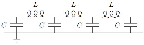
Figure 5.26:A circuit with three inductors.
Let us use the results of this section to study a finite example, with boundary conditions. Consider the circuit shown in Figure 5.26. This circuit in Figure 5.26 is analogous to the combination of springs and masses shown in Figure 5.27.
.](/physicsOfWaves/build/lt-33693-clipboard_e-c0c5e4837cc738b51e25ce446404a8a1.png)
Figure 5.27:A mechanical system analogous to Figure 5.26.
We already know that this is true for the middle. It remains only to understand the boundary conditions at the ends. If we label the inductors as shown in Figure 5.28, then we can imagine that this system is part of the infinite system shown in Figure 5.23, with the charges constrained to satisfy
This must be right. No charge can be displaced through inductors 0 and 4, because in Figure 5.26, they do not exist. This is just what we expect from the analogy to the system in 5.27, where the displacement of the 0 and 4 blocks must vanish, because they are taking the place of the fixed walls.
Now we can immediately write down the solution for the normal modes, in analogy with 5.21 and 5.22,
.](/physicsOfWaves/build/lt-33694-clipboard_e-6ab3175db406edf95affd4fcbe986b59.png)
Figure 5.28:A labeling of the inductors in Figure 5.26.
for = 1 to 3.
Forced Oscillation Problem for Coupled Circuits
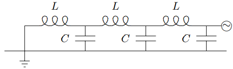
Figure 5.29:A forced oscillation with three inductors.
One more somewhat more practical example may be instructive. Consider the circuit shown in Figure 5.29. The  in Figure 5.29 stands for a source of harmonically varying voltage. We will assume that the voltage at this point in the circuit is fixed by the source, , to be
We would like to find the voltages at the other nodes of the system, as shown in Figure 5.30, with
We could solve this problem using the displaced charges, however, it is a little easier to use the fact that all the physical quantities in the infinite system in Figure 5.23 are proportional to in a mode with angular wave number . Because this is a forced oscillation problem (and because, as usual, we are ignoring possible free oscillations of the system and looking for the steady state solution), is determined from , by the dispersion relation for the infinite system of coupled circuits, 5.75.
The other thing we need is that
.](/physicsOfWaves/build/lt-33697-clipboard_e-9652cbf1b38a74486b9055d2490e3131.png)
Figure 5.30:The voltages in the system of Figure 5.29.
because the circuit is shorted out at the end. Thus we must combine the two modes of the infinite system, , into , and the solution has the form
We can satisfy the boundary condition at the other end by taking
This is the solution.
6This is not exactly true, however. Relativity imposes constraints. See chapter 11.
Problems
Zero does not work for because the eigenvalue equation has no solution.
See appendix .
More precisely, the string has a very large and nonlinear force constant for longitudinal stretching. The longitudinal oscillations have a much higher frequency and are much more strongly damped than the transverse oscillations, so we can ignore them in the frequency range of the transverse modes. See the discussion of the “light” massive spring in chapter 7.
Note also that, when is complex, the parts of the system do not all oscillate in phase, even though all oscillate at the same frequency.