In this chapter, we return to (9.46)-(9.48) and examine the consequences of Maxwell’s equations in a homogeneous material for a general traveling electromagnetic plane wave. The extra complication is polarization.
In most of our discussions of wave phenomena so far, we have assumed that the motion is taking place in a plane, so that we can draw pictures of the system on a sheet of paper. We have implicitly been restricting ourselves to two-dimensional waves. This is all right for longitudinal oscillations in three dimensions, because all the action is taking place along a single line. However, for transverse oscillations, going from two dimensions to three dimensions makes an enormous difference because there are two transverse directions in which the system can oscillate.
For example, consider a string in three dimensions, stretched in the z direction. Each point on the string can oscillate in both the x direction and the y direction. If the system were not approximately linear, this could be a horrendous problem. Linearity allows us to solve the problem of oscillation in the x-z plane separately from the problem of oscillation in the y-z plane. We have already solved these two-dimensional problems in chapter 5. Then we can simply put the results together to get the most general motion of the three-dimensional system. In other words, we can treat the x component of the transverse oscillation and the y component as completely independent.
Suppose that there is a harmonic traveling wave in the +z direction in the string. The displacement of the string at z from its equilibrium position, (0,0,z), can be written as
Ψ(z,t)=Re[(ψ1x^+ψ2y^)ei(kz−ωt)](12.1)
where x^ and y^ are unit vectors in the x and y direction and ψ1 and ψ2 are complex parameters describing the amplitude and phase of the oscillations in the x-z plane and the y-z plane,
ψj=Ajeiϕj for j=1 to 2.(12.2)
It is convenient to arrange these parameters into a complex vector
Z=(ψ1ψ2),(12.3)
which gives a complete description of the motion of the string.
“Polarization” refers to the nature of the motion of a point on the string (or other transverse oscillation). This motion is animated in program 12-1. You may want to read the discussion below with this program running.
If ϕ1=ϕ2, or A1 or A2 is zero, then 12.3 represent a linearly polarized string. Linear polarization is easy to understand. It means that each point on the string is oscillating back and forth in a fixed plane. For example,
u1=(10)(12.4)
u2=(01)(12.5)
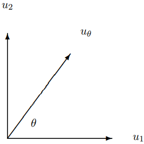
represent strings oscillating in the x-z plane and the y-z plane respectively. A string oscillating in a plane an angle θ from the positive x axis (towards the positive y axis) is represented by
uθ=(cosθsinθ).(12.6)
This is shown in the x-y plane in Figure 12.1. The polarization vectors 12.4-12.6 can be multiplied by a phase factor, eiϕ, without affecting the polarization state in any important way. This just corresponds to an overall resetting of the clock.
More interesting is circular polarization. A circularly polarized wave in a string is represented by either
(1i)(12.7)
or
(1−i).(12.8)
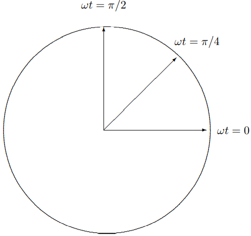
In 12.7, the y component lags behind the x component by π/2(=ϕ2). Thus, at any fixed point in space, the field rotates from x to y, or in the counterclockwise direction viewed from the positive z axis (with the wave coming at you), as shown in Figure 12.2. This is called “left-circular polarization” because the string resembles a left-handed screw. Likewise,
(1−i).(12.9)
represents clockwise rotation of the string. This is called “right-circular polarization.”
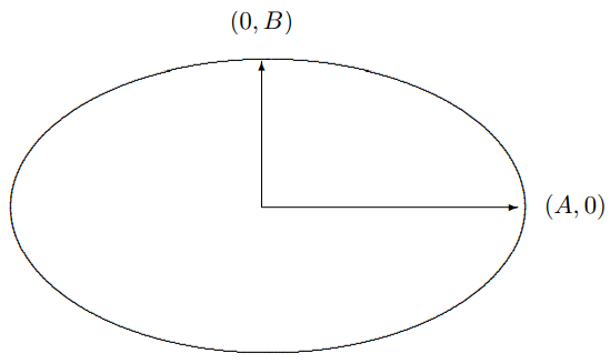
with A>B>0 represents elliptical polarization. A point on the string traces out an ellipse with semi-major axis A along the 1 axis and semi-minor axis B along the 2 axis, with counterclockwise rotation, as shown in Figure 12.3
Figure 12.3:Elliptical polarization with long axis in the x direction.
A completely general vector can be written in the following form:
(ψ1ψ2)=eiϕ(Acosθ−iBsinθAsinθ+iBcosθ)(12.11)
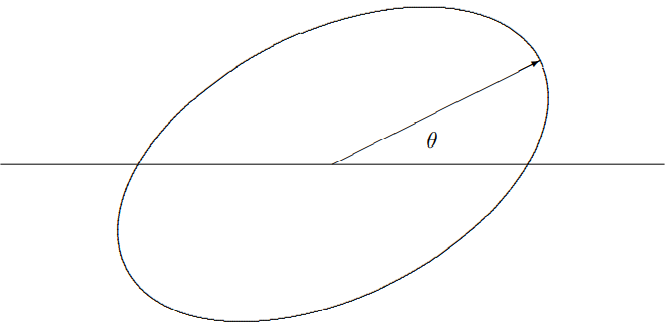
with A≥∣B∣ and 0≤θ<π and ϕ is real phase (which is not very relevant relevant to the physics but can be there to make the math look uglier). This represents elliptical polarization with semi-major axis A at an angle θ with the 1 axis, as in
uθ=(cosθsinθ).(12.12)
and semi-minor axis B as shown in Figure 12.4. If B is positive (negative), the rotation is counterclockwise (clockwise). The physically interesting parameters A, B and θ can be found from ψ1 and ψ2 as follows:
where the βs are determined by Maxwell’s equations to be
βy=cnεx,βx=−cnεy.(12.19)
As usual, we have written the wave with the irreducible time dependence, e−iωt. To get the real electric and magnetic fields, we take the real part of 12.14-12.15. Note, in particular, that the constants εj and βj for j=x and y may be complex.
The restriction to motion in the z direction is not important. Because the physics of Maxwell’s equations is invariant under rotations in three-dimensional space, we can write down the form of a plane wave moving with an arbitrary k vector by extracting the features of 12.14-12.17 that do not depend on the direction. These are:
k, E and B are mutually orthogonal vectors,
k⋅E=k⋅B=E⋅B=0;(12.20)
B is determined by the cross product
B=cnk^×E=ω1k×E,(12.21)
where k^ is a unit vector in the direction of the k vector, the direction of propagation of the wave.
These two conditions imply that a general real electromagnetic plane wave can be written as
E=Re(e(k)eik⋅r−iωt)B=Re(b(k)eik⋅r−iωt)(12.22)
where the vectors, e and b, are complex, in general, satisfying
b(k)=ω1k×e(k)=cnk^×e(k) and k^⋅e(k)=0.(12.23)
There are two things to note about the relations, 12.21.
It is enough to specify the direction of the electric field, e(k). The magnetic field is then determined by 12.21. The vector, e is called the “polarization” of the electromagnetic wave.
Because of 12.21, the polarization is perpendicular to k, and thus lives in a two-dimensional vector space.
In the two-dimensional space perpendicular to k, we can choose a basis of real vectors, e^1 and e^2, where
e^1⋅k^=e^2⋅k^=e^1⋅e^2=0,e^1×e^2=k^.(12.24)
For example, for a plane wave traveling in the z direction, k^=z^, we could take e1=x^ and e2=y^. Then we can write
e(k)=ψ1e^1+ψ2e^2.(12.25)
The components, ψ1 and ψ2 go into the the two-dimensional vector, 12.3, that describes the polarization state of the electromagnetic wave, just as it describes the polarization state of the string.[1] We can always go back to the components of the electric field using 12.23 and 12.20 and then find the magnetic field using 12.21.
Now the entire discussion of transverse waves on a string from 12.4 to 12.13 can be taken over to describe polarized light. The direction of displacement of the string goes over directly into the direction of the electric field. Thus the animation in program 12-1 applies just as well to the electric field in a polarized wave as to polarization in a string.
Because the energy density is a nonlinear function of the field strengths, we must use real fields in 12.24. The momentum density is
P=ϵE×B.(12.27)
The Poynting vector, a measure of energy flow, is
S=c2P.(12.28)
These quantities satisfy
∂t∂E+∇⋅S=0.(12.29)
The Poynting vector is useful because it measures the intensity of the wave, the energy per unit time per unit area carried by the electromagnetic wave. The relation, 12.27, then expresses conservation of energy. The sum of the change in the energy density at any point plus the energy flowing away from it is zero.
To see what these quantities look like in terms of the vector, Z, let us compute the electric and magnetic fields explicitly using 12.20 and 12.21:
You can check explicitly that 12.27 is satisfied. Because ω is very large for interesting electromagnetic waves, we are almost always interested in only the time averaged values of E and S. These are
⟨E⟩=8πϵ(A12+A22),(12.35)
⟨S⟩=k^μϵ8πc(A12+A22).(12.36)
Note that the time averaged values depend only on the quantity
∣Z∣2≡∣ψ1∣2+∣ψ2∣2=A12+A22.(12.37)
The intensity of the light is proportional to∣Z∣2.
Although linear polarization is more familiar and perhaps easier to understand, there is a sense in which circular polarization is the more fundamental. The plane electromagnetic wave in the k^ direction can be rotated around the k^ axis without changing anything but its polarization state. The rotation symmetry of the physics suggests that we ought to be able to find states that behave simply under such a rotation, and just get multiplied by a phase factor. These states are, in fact, the circular polarization states. The action of a rotation by an angle θ about the k^ axis on the polarization vector, Z, is represented by the matrix
Rθ=(cosθsinθ−sinθcosθ).(12.38)
For example, Rθ acting on u1, 12.4, gives uθ, 12.6:
Rθ(10)=(cosθsinθ).(12.39)
But on the left- and right-circularly polarized states,
Rθ(1i)=e−iθ(1i),Rθ(1−i)=eiθ(1−i).(12.40)
This is related to the fact that the circularly polarized states carry the maximum angular momentum possible, which in turn is related to the quantum mechanical property of the spin of the photon.
One reason that polarization is important is that the polarization state of an electromagnetic wave can be easily manipulated. Two of the most important devices for such manipulation are polarizers and wave plates.
In any beam of light, at any given point and time, the electric field points in a particular direction. Likewise, because any plane electromagnetic wave with a definite angular frequency can be described by 12.20 and 12.21,
EB=Re(e(k)eik⋅r−iωt)=Re(b(k)eik⋅r−iωt)(12.41)
b(k)=ω1k×e(k)=cnk^×e(k) and k^⋅e(k)=0.(12.42)
every plane wave is polarized. However, in an “unpolarized” beam, the light wave consists of a range of angular frequencies with different polarizations. As a result of the interference of the different harmonic components of the wave, the polarization wanders more or less randomly as a function of time and space, and on the average, no particular polarization is picked out. A simple example of what this looks like is animated in program 12-2, where we plot an electric field of the form
where the phases are random and the frequencies are chosen at random in a small range around a central frequency. You can watch the E field wandering in the x-y plane, eventually filling it up. The narrower the range of frequencies in the wave, the more slowly the polarization wanders. In the example in program 12-2, the range of frequencies is of the order of 10% of the central frequency, so the polarization wanders rapidly. But for a beam with a fairly well-defined frequency, the polarization will be nearly constant over many cycles of the wave. The time over which the polarization is approximately constant is called the coherence time of the wave. For a plane wave of definite frequency, the coherence time is infinite.
A “polarizer” is a device that allows light polarized in a particular direction (the “easy transmission axis” of the polarizer) to pass through with very little absorption, but absorbs most of the light polarized in the perpendicular direction. Thus an unpolarized light beam, passing though the polarizer, emerges polarized along the easy axis.
For the transverse oscillations of a string, a polarizer is simply a slit that allows the string to oscillate in one transverse direction but not in the perpendicular direction.
For electromagnetic waves, the most familiar example of a polarizer, Polaroid, was invented by Edwin Land over 50 years ago, partly in experiments done in the attic of the Jefferson Physical Laboratory, where he worked as an undergraduate at Harvard. The idea of polaroid is to make material that conducts electricity (poorly) in one direction, but not in the other. Then the electric field in the conducting direction will be absorbed (the energy going to resistive loss), while the electric field in the nonconductive direction will be unaffected. One way of doing this is to make sheets of polymer (polyvinyl alcohol) stretched (to align the polymer molecules along a preferred axis) and doped with iodine (to allow conduction along the polymer molecules).[2]
“Wave plates” are optical elements that change the relative phase of the two components of Z. Wave plates are possible because there are materials in which the index of refraction depends on the polarization. This property is called “birefringence.” It can happen in various ways.
For example, the transparent polymer material cellophane is made into thin sheets by stretching. Because of the stretching, the polymer strands tend to be oriented along the stretch direction. The dielectric constant in this material depends on the direction of the electric field. It is easier for charges to move along the polymer strands than across them. Thus the dielectric constant is larger for electric fields in the stretch direction.
The same effect may arise because of the inherent structure of a transparent crystal. An example is the naturally occurring mineral, calcite, a crystalline form of calcium carbonate, CaCO3. Crystals of calcite have the fascinating property of splitting a beam of unpolarized light into its two polarization states. Birefringence can even be produced mechanically, by stressing a transparent material, squeezing the electronic structure in one direction.
However the birefringence is produced, we can make a wave plate by orienting the material so that the x and y directions correspond to different indices of refraction, nx and ny, and then making a slice of the material in the form of a plate in the x-y plane, with some thickness ℓ in the z direction. Now an electromagnetic wave traveling in the z direction through the plate has different k values depending on its polarization:
k={cnxω for polarization in the x direction cnyω for polarization in the y direction (12.44)
In particular, the phase difference, between x and y polarized light in going through the plate is
Δϕ=cnx−nyωℓ.(12.45)
Note that in general the phase difference, Δϕ, depends on the frequency of the light. Even if nx and ny depend on frequency, it would be a bizarre accident if that dependence canceled the ω dependence from the explicit factor of ω in 12.39.
Figure 12.5:Initially unpolarized light passing through a pair of crossed polarizers with a wave plate in between.
Consider, now, putting such a wave plate between two crossed polarizers, oriented at ±45∘, as shown in Figure 12.5. Without the wave plate, no light would get through because the first polarizer transmits only light polarized at 45∘, described by the Z vector
Z=(1/21/2)(12.46)
and the second polarizer absorbs it.
Coming out of the first polarizer, the vector, Z, looks like 12.40 for all the frequency components in the white light. But when the wave plate is inserted in between, a frequency dependent phase difference is added, so that the Z vector coming out of the wave plate (up to an irrelevant overall phase) looks like
Z=(1/2e−iΔϕ/2).(12.47)
For frequencies such that e−iΔϕ is −1, the light is polarized in the −45∘ direction, and gets e−iΔϕ through the second polarizer without further attenuation. But for frequencies such that e is 1, the light is still absorbed by the second polarizer. Intermediate frequencies are partially absorbed.
It is this frequency dependence that produces the interesting patterns of color that you see when you put cellophane or a stressed piece of plastic between polarizers.
The effects of wave plates and polarizers and the like can be summarized by multiplication of the Z vector by 2×2 matrices. For example, a perfect polarizer with an axis at an angle θ from the 1 axis can be represented by
Pθ=(cos2θcosθsinθcosθsinθsin2θ).(12.48)
The object Pθ is called a “projection operator,” because it projects the vector onto the direction parallel to uθ. It satisfies
PθPθ=Pθ,(12.49)
as it must, since the first polarizer produces polarized light and the second one transmits it perfectly. Pθ acting on a vector transmits the component in the θ direction. This is easiest to visualize if θ=0 or π/2. The matrices
P0=(1000),Pπ/2=(0001),(12.50)
represent polarizers along the 1 and 2 axes respectively.
A wave plate in which the phase difference is π/2 is called a “quarter wave plate.” For a wave plate in which the phase difference is between 0 and π, it is conventional to call the axis with the smaller phase the “fast axis.” A quarter wave plate with fast axis along the 1 axis is represented by
Q0=(100i).(12.51)
Notice that we can write
Q0=P0+iPπ/2.(12.52)
This should convince you that in general if the fast axis is in the θ direction, the quarter wave plate looks like
Qθ=Pθ+iPθ+π/2.(12.53)
The discussion of 12.39 shows that in general, a wave plate will only be a quarter wave plate for light of a definite frequency.
A wave plate in which the phase difference is π is called a “half wave plate.” A half wave plate is obtained by replacing the i in 12.45-12.47 by -1. Thus,
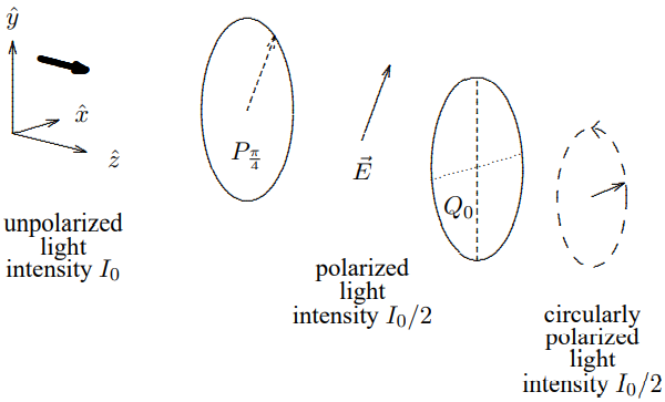
Here are two amusing devices that you can make with these optical elements (or matrices). Consider the combination of first a polarizer at 45∘ and then a quarter wave plate, as shown in Figure 12.6. By forming the matrix product, Q0Pπ/4, you can see that this produces counterclockwise circularly polarized light from anything with a component of polarization in the π/4 direction. The argument goes like this. The product is
When this acts on an arbitrary vector you get circularly polarization unless the vector is annihilated by Pπ/4.
Q0Pπ/4(ψ1ψ2)=2ψ1+ψ2(1i).(12.57)
In the opposite order, Pπ/4Q0 is an analyzer for circularly polarized light. It annihilates counterclockwise light and converts clockwise polarized light to light linearly polarized in the π/4 direction.
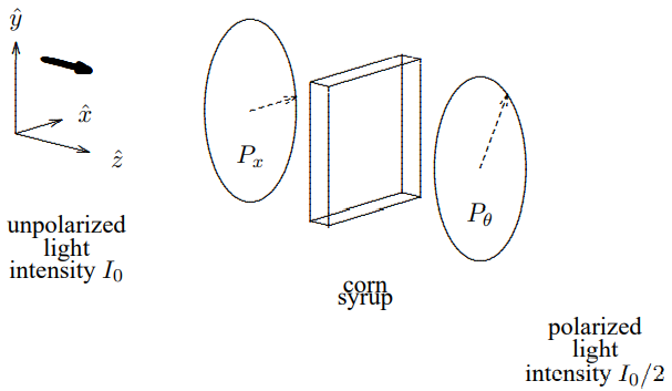
“Optical activity” is a property of many organic and some inorganic compounds. An optically active material rotates the polarization of light without absorbing either component of the polarization. A familiar example of such a material is corn syrup, a thick aqueous solution of sugar that you probably have in your kitchen. If you put a rectangular container of corn syrup between polarizers, as shown in Figure 12.7, and rotate the second polarizer until the intensity of the light getting through is a maximum, you will find that direction of the second polarizer is not the same as that of the first. The plane of the polarization has been rotated by some angle θ. The rotation angle, θ, is proportional to the thickness of the container, the length of the region of syrup that the light goes through.
Figure 12.7:A rectangular container of corn syrup between polarizers.
Clearly, the optical activity of corn syrup cannot depend on crystal structure, because the stuff is a perfectly uniform liquid, completely invariant under rotations in three-dimensional space. It can have no special axes, or any such thing. Optical activity must work very differently from birefringence.
You can find a clue to the nature of optical activity by considering what it looks like if you look at it in a mirror. If you reflect the system illustrated in Figure 12.7 in the x-z plane, by changing the sign of all the y coordinates, the angle θ changes to −θ. Thus the corn syrup that you see in a mirror must be fundamentally different from the corn syrup in your kitchen. This is not so strange. After all, your right hand looks like a left hand when you look at it in a mirror. The corn syrup must have the same property and have a definite “handedness.” In fact, because of the tetrahedral bonding of the carbon atoms of which they are built, the sugar molecules in the corn syrup can and do have such a handedness.
Because of the handedness of the sugar molecules, the index of refraction of the corn syrup actually depends on the handedness of the light. It is slightly different for left- and right-circularly polarized light. This happens because the E field of a circularly polarized beam twists slightly as it traverses each sugar molecule and sees a slightly different electronic structure depending on the direction of the twist. Then, because the indices of refraction are slightly different, the left- and right-circularly polarized components of the light get different phase factors (kℓ) in passing through a thickness, ℓ, of the syrup.
We can now use our matrix language to see how this leads to optical activity. Up to an irrelevant overall phase, we can choose the phase produced on the left-circularly polarized light to be −θ and that on the right-circularly polarized light to be θ. Then we can represent the action of the syrup on an arbitrary wave by the matrix
e−iθP++eiθP−,(12.58)
where P± are matrices that pick out the left- and right-circularly polarized components, respectively. They satisfy
This is just the rotation matrix Rθ, of 12.34! Rθ rotates both components of any light by an angle θ.
One might wonder about the reason for the handedness of the sugar molecules. In fact, there are physical processes, the weak interactions that give rise to β-radioactivity, that look different when reflected in a mirror[3] and thus in principle could distinguish between left-handed and right-handed molecules. However, these interactions are most likely irrelevant to the handedness of corn syrup. Probably, the reason is biology rather than physics. Long ago, when the beginnings of life emerged from the primordial soup, purely by accident, the right-handed sugars were used. From then on, the handedness was maintained by the processes of reproduction.
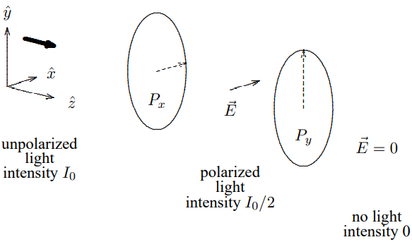
Figure 12.8:Initially unpolarized light passing through a pair of crossed polarizers.
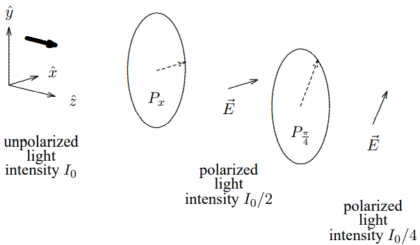
Polarization offers many opportunities to get confused when you think of the light wave in terms of photons. Let us imagine turning down the intensity of the light to the point where one photon at a time is going through the polarizers and consider first the deceptively simple situation of light moving in the z direction through crossed polarizers in the x-y plane. Suppose that the first polarizer transmits light polarized in the x direction, and the second transmits light polarized in the y direction. This is deceptively simple because it seems that we can interpret what is going on simply in terms of photons. The situation is depicted in Figure 12.8. This seems simple enough to interpret in terms of photons. The unpolarized light in region I is composed equally of photons polarized in the x direction and in the y direction (goes the wrong “classical” argument). Those polarized in the x direction get through the first polarizer, so half the photons are still around in region II, where the intensity is reduced by half. Then none of these get through the second polarizer, so that the intensity in region III is zero.
But compare this with the apparently similar situation in which the second polarizer transmits light polarized at 45∘ in the x-y plane, as shown in Figure 12.9. Now the wave description tells us that the intensity in region III is reduced by another factor of 2 from that in region II. This is impossible to interpret in terms of classical particles. To see this, it is only necessary to turn down the intensity so that only one photon comes through at a time. Then the first polarizer is OK. As before, if the photon is polarized in the x direction, it get through. But now what happens at the second polarizer. The photon cannot split up. Either it gets through or it doesn’t. To be consistent with the wave description, in which the intensity is reduced by another factor of two, the transmission at the second polarizer must be a probabilistic event. Half the time the photon gets through. Half the time it is absorbed. There is no way for the
Figure 12.9:Initially unpolarized light passing through a pair of polarizers at with axes at 45∘.
photon in region II to tell whether it is going to make it! It is random. God plays dice.
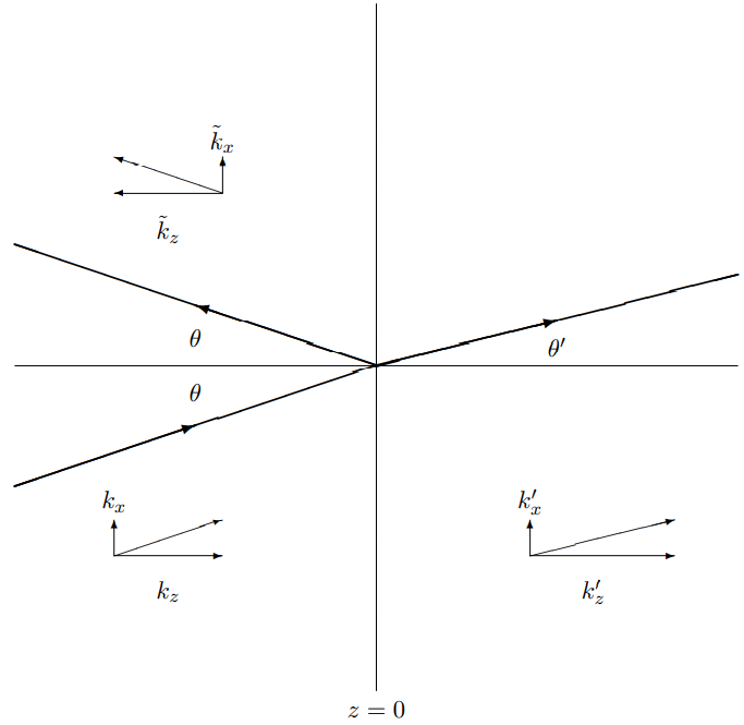
Let us return to the infinite plane boundary between two dielectrics that we discussed in chapter 9, but now consider an electromagnetic wave coming in at an arbitrary angle. As in chapter 5, we will assume that the boundary is the z=0 plane, and that for z<0 we have dielectric constant ϵ, while for z>0, dielectric constant ϵ′. We assume μ=1 everywhere.
On the general grounds of translation invariance and local interactions discussed in the previous chapter, all the components of the electric and magnetic fields will have the general form
ψ(r,t)∝eik⋅r+Reik⋅rψ(r,t)∝τeik′⋅r for z≤0 for z≥0(12.62)
where
k~x=kx,kx′=kx,(12.63)
and
k~z=−ω2/v2−kx2=−kzkz′=ω2/v′2−kx2.(12.64)
Thus Snell’s law is satisfied, with θ and θ′ defined as shown in Figure 12.10.
Figure 12.10:Scattering of plane waves from a plane boundary.
The details of the scattering will depend on the polarization. It is clear (by symmetry as usual) that the two cases will be polarization in the x-z plane and polarization perpendicular to the x-z plane. Of course, we lose nothing by considering these two separately, because of linearity. Any polarization for the incoming wave can be dealt with by forming a linear combination of the parallel and perpendicular solutions.
Polarization Perpendicular to the Scattering Plane
Let us first consider perpendicular polarization. This means that the electric field is in the y direction (out of the plane of the paper), while the magnetic field is the x-z plane:4
Ey(r,t)=Aei(kr−ωt)+R⊥Aei(k~⋅r−ωt) for z≤0Ey(r,t)=τ⊥Aei(k′⋅r−ωt) for z≥0Ez=Ex=0(12.66)
Bx(r,t)=−cnAcosθei(k⋅r−ωt)+cncosθR⊥Aei(k⋅r−ωt)Bx(r,t)−−cn′cosθ′τ⊥Aei(k′⋅r−ωt)Bz(r,t)=cnsinθAei(k⋅r−ωt)+cnsinθR⊥Aei(k⋅r−ωt)Bz(r,t)=cn′sinθ′τ⊥Aei(k′⋅r−ωt)By=0 for z≤0 for z≥0 for z≤0 for z≥0(12.68)
The system is shown in Figure 12.11. This figure shows the directions of the magnetic fields of the incoming (Bi), reflected (Br), and transmitted (Bt) component waves in scattering of an electromagnetic plane wave polarized parallel to a plane dielectric boundary. The k vectors are shown directly beneath the magnetic fields. The nontrivial boundary conditions are that Ey and Bx are continuous (the latter because we have assumed μ=1 so there is no sheet of bound current on the boundary). Bz is also continuous, but that provides no new information. Thus
By(r,t)=Aei(k⋅r−ωt)+R∥Aei(k⋅r−ωt)By(r,t)=τ∥Aei(k′⋅r−ωt)Bz=Bx=0, for z≤0 for z≥0(12.71)
where, for convenience, we have defined the reflection and transmission coefficients in terms of the magnetic fields, and
Ex(r,t)=nccosθAei(k⋅r−ωt)−nccosθR∥Aei(−k⋅r−ωt)Ex(r,t)=n′ccosθ′τ∥Aei(k′⋅r−ωt)Ez(r,t)=−ncsinθAei(k⋅r−ωt)−ncsinθR∥Aei(−k~⋅r−ωt)Ez(r,t)=−n′csinθ′τ∥Aei(k′⋅r−ωt)Ez=0. for z≤0 for z≥0 for z≤0 for z≥0(12.72)
Now the nontrivial boundary conditions are the continuity of By and Ex. Ez is not continuous because a surface bound charge density builds up on the dielectric boundary. The boundary conditions yield
1+R∥=τ∥(12.73)
ncosθ(1−R∥)=n′cosθ′τ∥(12.74)
or
τ∥=1+ξ∥2(12.75)
R∥=1+ξ∥1−ξ∥(12.76)
where
ξ∥=cosθ/ncosθ′/n′=n′2kzn2kz′.(12.77)
One of the interesting things about 12.74 is that when
n′2kzn2kz′−1(12.78)
there is no reflection. This condition is satisfied for a special angle of incidence called Brewster’s angle. We can understand the significance of Brewster’s angle as follows:
from Snell’s law, n′2n2−sin2θsin2θ′(12.79)
kzkz′=kx′/kz′kx/kz=tanθ′tanθ(12.80)
n′2kzn2kz′=sinθcosθsinθ′cosθ′=1.(12.81)
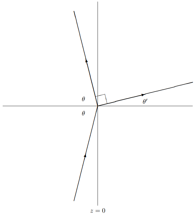
Thus sin2θ=sin2θ′. Because θ=θ′ (that would be the trivial situation with no boundary), this means that
θ=π/2−θ′.(12.82)
In other words, Brewster’s angle is defined by the condition that the reflected and transmitted plane waves are perpendicular, as shown in the diagram in Figure 12.12. The relevance of this condition is that the reflected wave can be thought of as being produced by the motion of the charges on the boundary. But if these are moving in a direction perpendicular to the electric field in the would-be reflected wave, then the wave cannot be produced.
Because Maxwell’s equations are partial differential equations, lots of initial conditions or boundary conditions must be specified to determine the solutions. For example, a constant electric field everywhere is a solution to the free-space Maxwell’s equations, and therefore you can add a constant field to any solution and it will still be a solution. Such things must be determined by physical initial conditions or boundary conditions. One set of conditions that is frequently interesting is an analog of the boundary condition at infinity that we discussed for one-dimensional waves. Suppose that you have a universe which is initially stationary, with no electric currents, no magnetic fields, and only electric fields due to stationary charges (which you know how to compute from Physics 15b). At some time, you begin to move charges around in some finite region of space. What are the electric and magnetic fields produced in this way? This question has a relatively simple answer that is a nice intuitive generalization of the relations you learned in 15b for the electric and vector potentials from stationary charge and current distributions. These relations were
ϕ(r)=∫d3r′∣∣r−r′∣∣ρ(r′)(12.83)
A(r)=c1∫d3r′∣∣r−r′∣∣J(r′)(12.84)
The generalizations are
ϕ(r,t)=∫d3r′∣r−r′∣ρ(r′,t−∣r−r′∣/c)(12.85)
A(r,t)=c1∫d3r′∣∣r−r′∣∣J(r′,t−∣r−r∣/c)(12.86)
It is a straightforward, but tedious, exercise in vector calculus to show these satisfy Maxwell’s equations. I am not going to talk about this (I’ll write down the derivation in an appendix for those of you who are interested), but it is worth trying to understand what these relations mean physically. The important physical point that these relations imply is that if the charge and current distributions depend on time, and if they are producing the fields, then what determines what the field is at some point r is the values of the charge and current distributions at earlier times. The farther away the charge is, the earlier the time has to be. That is what the factor of t−∣r−r′∣/c is telling us. The appearance of this factor is a kind of boundary condition at infinity. It is consistent with the relativistic version of the principle of causality. Because information cannot be transferred faster than light, a charge distribution at a space-time point (r′,t′) can effect the fields at the space-time point (r,t), only if t≥t′ and
t−t′∣r−r′∣≤c(12.87)
In these relations, 12.82 and 12.83, however, the condition is even stronger — a charge distribution at a space time point (r′,t′) can effect the fields at the space time point (r,t) only if light can travel directly from (r′,t′) to (r,t) — that is ift≥t′ and
ck (12.88)
or
t−t′=∣∣r−r′∣∣/c(12.89)
or
t′=t−∣r−r′∣/c(12.90)
These are just words. We have not derived this! The real justification of this discussion comes when you check that the relations actually satisfy Maxwell’s equations. That can wait for Physics 153 or 232 (or the appendix if you are in a hurry). However, I hope that this discussion at least makes the result reasonable. In fact you have already seen the result in action in 15b in Purcell’s discussion of the electric field from a charge that starts and stops. Look at the ANIMATIONS - PURCELL - the field from a charge that suddenly accelerates. This is an animation of a famous figure in Purcell’s book. The interesting thing about the animation is the kink in the electric field that propagates out from the acceleration event at the velocity of light — because it is light. Inside the kink, the fields are those of the moving charge. Outside the kind, the fields are those of the stationary charge. The kink — the electromagnetic way — is what connects the two asymptotic regions together. It is also fun to compare with PURCELL2 which illustrates what happens if an initially moving charge stops suddenly.
Now let’s see at what the electric and magnetic fields look like in an important limit. The connection between the potentials and the fields is the following:
E=−∇ϕ−c1∂t∂A(12.91)
B=∇×A(12.92)
These relations are completely general. The special limit that I want to consider is one in which the charges and currents are confined to a small region around r=0. Then we will look at the electric and magnetic fields produced by the moving charges far away, for large ∣r∣. It is actually easiest to look at the magnetic field:
B=∇×A=∇×c1∫d3r′∣r−r′∣J(r′,t−∣r−r′∣/c)(12.93)
The point is that the curl (∇×) can operate in two different places, either on the 1/∣∣r−r′∣∣ or on the −∣∣r−r′∣∣/c in the time dependence of J. The first gives a contribution that drops of like 1/r2 for large r, just like the magnetic field from a time-independent distribution of currents. But the second gives a contribution that only falls off like 1/r. Thus this contribution dominates for large r. Explicitly (using the chain rule), it is
where in 12.92 we have dropped a r′ in the numerator because this term falls like 1/r2 for large r.
This is the magnetic field of an electromagnetic wave. Notice that it is perpendicular to the direction of motion (r^). The 1/r fall-off is what we expect for an electromagnetic wave, because the energy density goes like the square of the field, and falls off like 1/r2 as the wave spreads.
The electric field can be computed in a similar way, although you also need to use the conservation of electric charge.
∂t∂ρ+∇⋅J=0(12.96)
As you would expect, the result is that the electric field has the same magnitude as the magnetic field and is perpendicular to both direction of motion and to the magnetic field. The piece that corresponds to a traveling electromagnetic wave can be written as
The reason for the restriction to nonrelativistic motion of charges is that if a charged particle is moving at a speed close to the velocity of light, then we cannot neglect its position, r′, when it is moving towards r. To see this, consider the impossible limit in which the charge is moving towards the point r at the speed of light. Then if the charge contributes to the electric field at r at one time, then it also contributes at later times because the particle keeps up with the moving light wave. While v=c is impossible, for v≈c, the r′ dependence cannot be ignored because it leads to very rapid time dependence of the potentials, and hence to large fields. What happens is that the contribution of charges moving relativistically to the electric fields in front of them get enhanced by factors of c−vc. This effect is widely used today to produce intense “light” from particle accelerators — so called synchrotron radiation. You can see this effect in the ANIMATIONS if you make v close to 1.
A particularly important and instructive case of 12.97 is the nonrelativistic motion of a single charge, Q, moving along a trajectory R(t). For this system,5
Then the integration over d3r′ in (a) eliminates the δ-function, and the electric field of the outgoing electromagnetic wave is proportional to the acceleration,
E(r,t)≈c21r1Qr^×(r^×a(t−r/c))(12.102)
where
a(t)=dt2d2R(l)(12.103)
All that the cross products with r^ do is to pick out minus the component of a(l−r/c) that is perpendicular to r. It follows from the famous “bac-cab” identity,
This had to happen because the electric field of an electromagnetic wave is perpendicular to its direction of motion. In this case, for large r, the wave is nearly a plane wave moving in direction r.
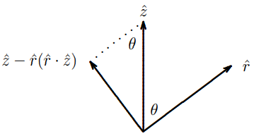
The vector z^−r^(r^⋅z^) is the component of z^ perpendicular to r, as illustrated in Figure 12.13.
Figure 12.13:Evidently, the magnitude of z^−r^(r^⋅z^) is sinθ. This means that the intensity of the electromagnetic wave at an angle θ from the z axis is proportional to sin2θ. The intensity pattern can be conveniently represented in polar coordinates, where we plot the intensity as a function of θ. The result is shown below. This is the “antenna pattern” for the oscillating
Figure 12.14:dipole in the z direction. It is shown in Figure 12.14. The two lobes of the pattern arise because the field is highest in the x-y plane, for θ=π/2, and drops to zero as we approach the z axis, θ=0 or θ=π.
These things are called retarded potentials. This is a confusing name, since there is really nothing special about the potentials themselves. What is special is the assumption of a particular relation between the potentials and the charges and currents — that the fields are being produced entirely by the charges and currents. Here I show that they satisfy Maxwell’s equations. I call this an appendix because you are NOT responsible for knowing the details. I include it for your general education.
Some mathematical things to notice about the solution:
i and ii come from a (from the ∂t2∂2 and −∇2 terms respectively) and iii comes from b. Now the ∇ in ii gives two terms — acting on ρ˙ cancels i and acting on cancels iii. Thus
∇⋅E=4πρ.(12.124)
Likewise,
∇×B−c1∂t∂E(12.125)
=∇×(∇×A)−c1∂t∂(−∇ϕ−c1∂t∂A)(12.126)
=∇(∇⋅A)−∇2A−∇(c1∂t∂ϕ)+c21∂t2∂2A
or using the Lorentz gauge condition,
=(−∇2+c21∂t2∂2)A
Form here on, the derivation is the same as for ∇⋅E, and we find
∇×B−c1∂t∂E=c4πJ
QED.
5 This equation makes use of δ-function notation. To a physicist, a δ-function δ(x) is just a function that has area 1 and is so sharply peaked around x = 0 that we don’t care exactly what it looks like. All that matters is the area and where the peak is. The δ3 ~ ¡ ~r − R(t) ¢ in the equation is actually the product of three delta functions, for the x, y and z components, and just tells you that ~r = (x, y, z) = R~(t) = ¡ X(t), Y (t), Z(t) ¢ — that is that the particle is moving along the trajectory R~(t). For a mathematical discussion of the δ-function you can look at http://mathworld.wolfram.com/DeltaFunction.html. But don’t be frightened. It is just a simple device for ignoring small details that we don’t care about. If you translate the integral into words or pictures, it may help.

 12-1
12-1 12-2
12-2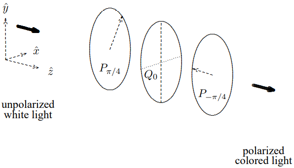
. The two lobes of the pattern arise because the field is highest in the x-y plane, for \theta=\pi / 2, and drops to zero as we approach the z axis, \theta = 0 or \theta = \pi.](/physicsOfWaves/build/lt-32980-clipboard_e-9e62cbad019f05b56c74867a99643893.png)