Traveling waves with a definite frequency carry energy but no information. They are just there, always have been and always will be. To send information, we must send a nonharmonic signal.
10.1: Signals in Forced Oscillation
Pulse on a String
 10-1
10-1
We begin with the following illustrative problem: the transverse oscillations of a semiinfinite string stretched from to , driven at with some arbitrary transverse signal , and with a boundary condition at infinity that there are no incoming traveling waves. This simple system is shown in Figure 10.1.

Figure 10.1:A semiinfinite string.
There is a slick way to get the answer to this problem that works only for a system with the simple dispersion relation,
The trick is to note that the dispersion relation, 10.1, implies that the system satisfies the wave equation, 6.4, or
It is a mathematical fact (we will discuss the physics of it below) that the general solution to the one-dimensional wave equation, 10.2, is a sum of right-moving and left-moving waves with arbitrary shapes,
where and are arbitrary functions. You can check, using the chain rule, that 10.3 satisfies 10.2,
Given this mathematical fact, we can find the functions and that solve our particular problem by imposing boundary conditions. The boundary condition at infinity implies
because the function describes a wave moving in the direction. The boundary condition at implies
which gives
This describes the signal, , propagating down the string at the phase velocity with no change in shape.
For the simple function
the shape of the string at a sequence of times is shown in Figure 10.2 and animated in program 10-1.
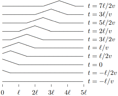
Figure 10.2:A triangular pulse propagating on a stretched string.
Fourier integrals
Let us think about this problem in a more physical way. In the process, we will understand the physics of the general solution, 10.3. This may seem like a strange thing to say in a section entitled, “Fourier integrals.” Nevertheless, we will see that the mathematics of Fourier integrals has a direct and simple physical interpretation.
The idea is to use linearity in a clever way to solve this problem. We can take apart into its component angular frequencies. We already know how to solve the forced oscillation problem for each angular frequency. We can then take the individual solutions and add them back up again to reconstruct the solution to the full problem. The advantage of this procedure is that it works for any dispersion relation, not just for 10.1.
Because there may be a continuous distribution of frequencies in an arbitrary signal, we cannot just write as a sum over components, we need a Fourier integral,
The physics of 10.9 is just linearity and time translation invariance. We know that we can choose the normal modes of the free system to have irreducible exponential time dependence, because of time translation invariance. Since the normal modes describe all the possible motions of the system, we know that by taking a suitable linear combination of normal modes, we can find a solution in which the motion of the end of the system is described by the function, . The only subtlety in 10.9 is that we have assumed that the values of that appear in the integral are all real. This is appropriate because a nonzero imaginary part for in describes a function that goes exponentially to infinity as . Physically, we are never interested in such things. In fact, we are really interested in functions that go to zero as . These are well-described by the integral over real , 10.9.
Note that if is real in 10.9, then
thus
It is actually easier to work with the complex Fourier integral, 10.9, with the irreducible complex exponential time dependence, than with real expansions in terms of and . But you may also see the real forms in other books. You can always translate from 10.9 by using the Euler identity
For each value of , we can write down the solution to the forced oscillation problem, incorporating the boundary condition at . Each frequency component of the force produces a wave traveling in the direction.
then we can use linearity to construct the solution by adding up the individual traveling waves from 10.13 with the coefficients from 10.9. Thus
where and are related by the dispersion relation.
Equation 10.14 is true quite generally for any one-dimensional system, for any dispersion relation, but the result is particularly simple for a nondispersive system such as the continuous string with a dispersion relation of the form 10.1. We can use 10.1 in 10.14 by replacing
Note that while is determined by the dispersion relation, the sign of , for a given , is determined by the boundary condition at infinity. and must have the same sign, as in 10.15, to describe a wave traveling in the direction. Putting 10.15 into 10.14 gives
Comparing this with 10.9 gives 10.7.
Let us try to understand what is happening in words. The Fourier integral, 10.9, expresses the signal as a linear combination of harmonic traveling waves. The relation, 10.15, which follows from the dispersion relation, 10.1, and the boundary condition at , implies that each of the infinite harmonic traveling waves moves at the same phase velocity. Therefore, the waves stay in exactly the same relationship to one another as they move, and the signal is never distorted. It just moves with the waves.
The nonharmonic signal is called a “wave packet.” As we have seen, it can be taken apart into harmonic waves, by means of the Fourier integral, 10.9.
10.2: Dispersive Media and Group Velocity
For any other dispersion relation, the signal changes shape as it propagates, because the various harmonic components travel at different velocities. Eventually, the various pieces of the signal get out of phase and the signal is dispersed. That is why such a medium is called “dispersive.” This is the origin of the name “dispersion relation.”
Group Velocity
 10-2
10-2
If you are clever, you can send signals in a dispersive medium. The trick is to send the signal not directly as the function, , but as a modulation of a harmonic signal, of the form
where is the signal. Very often, you want to do this anyway, because the important frequencies in your signal may not match the frequencies of the waves with which you want to send the signal. An example is AM radio transmission, in which the signal is derived from sound with a typical frequency of a few hundred cycles per second (Hz), but it is carried as a modulation of the amplitude of an electromagnetic radio wave, with a frequency of a few million cycles per second.[1]
You can get a sense of what is going to happen in this case by considering the sum of two traveling waves with different frequencies and wave numbers,
where
for
The sum can be written as a product of cosines, as
Because of 10.20, the first factor varies slowly in and compared to the second. The result can be thought of as a harmonic wave with frequency with a slowly varying amplitude proportional to the first factor. The space dependence of 10.21 is shown in Figure 10.3.
 for t = 0 and k0/ks = 10.](/physicsOfWaves/build/lt-33395-clipboard_e-c86eb944530c614ccb46eb7a8a7a123e.png)
Figure 10.3:The function 10.21 for t = 0 and k0/ks = 10.
You should think of the first factor in 10.21 as the signal. The second factor is called the “carrier wave.” Then 10.21 describes a signal that moves with velocity
while the smaller waves associated with the second factor move with velocity
These two velocities will not be the same, in general. If 10.20 is satisfied, then (as we will show in more detail below) will be roughly the phase velocity. In the limit, as becomes very small, 10.22 becomes a derivative
This is called the “group velocity.” It measures the speed at which the signal can actually be sent.
The time dependence of 10.21 is animated in program 10-2. Note the way that the carrier waves move through the signal. In this animation, the group velocity is smaller than the phase velocity, so the carrier waves appear at the back of each pulse of the signal and move through to the front.
Let us see how this works in general for interesting signals, . Suppose that for some range of frequencies near some frequency , the dispersion relation is slowly varying. Then we can take it to be approximately linear by expanding in a Taylor series about and keeping only the first two terms. That is
and the higher order terms are negligible for a range of frequencies
where is a constant that depends on and the details on the higher order terms. Then you can send a signal of the form
(a complex form of 10.17, above) where satisfies 10.9 with
This describes a signal that has a carrier wave with frequency , modulated by the interesting part of the signal, , that acts like a time-varying amplitude for the carrier wave, . The strategy of sending a signal as a varying amplitude on a carrier wave is called amplitude modulation.
Usually, the higher order terms in 10.25 are negligible only if . If we neglect them, we can write 10.25 as
where and are constants we can determine from 10.25,
and is the group velocity
For the signal 10.28
Thus 10.14 becomes
but then 10.29 gives
The modulation travels without change of shape at the group velocity given by 10.32, as long as we can ignore the higher order term in the dispersion relation. The phase velocity
has nothing to do with the transmission of information, but notice that because of the extra in 10.35, the carrier wave travels at the phase velocity.
You can see the difference between phase velocity and group velocity in your pool or bathtub by making a wave packet consisting of several shorter waves.
10.3: Bandwidth, Fidelity, and Uncertainty
The relation 10.9 can be inverted to give in terms of as follows
This is the “inverse Fourier transform.” It is very important because it allows us to go back and forth between the signal and the distribution of frequencies that it contains. We will get this result in two ways: first, with a fancy argument that we will use again and explain in more detail in chapter 13; next, by going back to the Fourier series, discussed in chapter 6 for waves on a finite string, and taking the limit as the length of the string goes to infinity.
The fancy argument goes like this. It is very reasonable that the integral in 10.37 is proportional to because if we insert 10.9 and rearrange the order of integration, we get
The integral averages to zero unless . Thus the integral is simply proportional to times a constant factor. The factor of can be obtained by doing some integrals explicitly. For example, if
for then, as we will show explicitly in 10.49-10.56, 10.37 yields
which can, in turn, be put back in 10.9 to give 10.39. For , the integral can be done by the trigonometric substitution :
To get the inverse Fourier transform, 10.37, as the limit of a Fourier series, it is convenient to use a slightly different boundary condition from those we discussed in chapter 6, fixed ends and free ends. Instead, let us consider a string stretched from to , in which we assume that the displacement of the string from equilibrium at is the same as the displacement at ,2
The requirement, 10.42, is called “periodic boundary conditions,” because it implies that the function that describes the displacement of the string is periodic in with period . The normal modes of the infinite system that satisfy 10.42 are
for integer , because changing by in 10.43 just changes the phase of the exponential by . Thus if is an arbitrary function satisfying , we should be able to expand it in the normal modes of 10.43,
Likewise, for a function , satisfying for some large time , we expect to be able to expand it as follows
where we have changed the sign in the exponential to agree with 10.9. We will show that as , this becomes equivalent to 10.9.
Equation 10.44 is the analog of 6.8 for the boundary condition, 10.42. The sum runs from to rather than 0 to because the modes in 10.43 are different for and . For this Fourier series, the inverse is
where we have used the identity
Now suppose that goes to 0 for large (note that this is consistent with the periodic boundary condition 10.42) fast enough so that the integral in 10.46 is well defined as for all . Then because of the factor of in 10.47, the all go to zero like . Thus we should multiply by to get something finite in the limit. Comparing 10.45 with 10.9, we see that we should take to be .
Thus the relation, 10.45, is an analog of the Fourier integral, 10.9 where the correspondence is
In the limit, , the sum becomes an integral over .
Multiplying both sides of 10.46 by , and making the substitution of 10.48 gives 10.37.
Solvable Example
For practice in dealing with integration of complex functions, we will do the integration that leads to 10.40 in gory detail, with all the steps.
First we get rid of the absolute value —
and write the second integral as an integral from 0 to —
but we know how to differentiate even complex exponentials (see the discussion of 3.108), so we can write
Thus
or, using the fundamental theorem of integral calculus,
This function of is called a “pole.” While the function is perfectly well behaved for real , it blows up for , which is called the position of the pole in the complex plane. Now we just have to add the complex conjugate to get
which is 10.40. We already checked, in 10.41, that the factor of makes sense.
The pair 10.39-10.40 illustrates a very general fact about signals and their associated frequency spectra. In Figure 10.4 we plot for and and in Figure 10.5, we plot for the same values of . Notice that as increases, the signal becomes more sharply peaked near but the frequency spectrum spreads out. And conversely if ¡ is small so that is sharply peaked near , then is spread out in time. This complementary behavior is general. To resolve short times, you need a broad spectrum of frequencies.
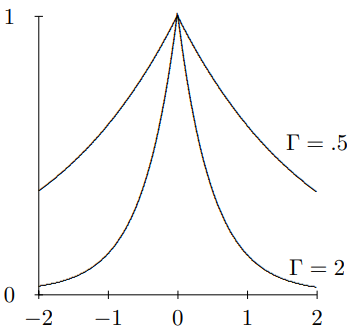
Figure 10.4: for and .
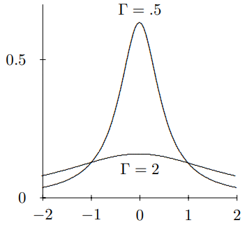
Figure 10.5: for the same values of .
Broad Generalities
We can state this fact very generally using a precise mathematical definition of the spread of the signal in time and the spread of the spectrum in frequency.
We will define the intensity of the signal to be proportional to . Then, we can define the average value of any function weighted with the signal’s intensity as follows
This weights most when the signal is most intense.
For example, is the average time, that is the time value around which the signal is most intense. Then
measures the mean-square deviation from the average time, so it is a measure of the spread of the signal.
We can define the average value of a function of in an analogous way by integrating over the intensity of the frequency spectrum. But here is the trick. Because of 10.9 and 10.37, we can go back and forth between and at will. They carry the same information. We ought to be able to calculate averages of functions of by using an integral over . And sure enough, we can. Consider the integral
This shows that multiplying by is equivalent to differentiating the corresponding and multiplying by .
Thus we can calculate as
and
is a measure of the spread of the frequency spectrum, or the “bandwidth.”
Now we can state and prove the following result:
One important consequence of this theorem is that for a given bandwidth, , the spread in time of the signal cannot be arbitrarily small, but is bounded by
The smaller the minimum possible value of you can send, the higher the “fidelity” you can achieve. Smaller means that you can send signals with sharper details. But 10.63 means that the smaller the bandwidth, the larger the minimum , and the lower the fidelity.
To prove 10.62 consider the function3
which depends on the entirely free parameter . Now look at the ratio
This ratio is obviously positive, because the integrands of both the numerator and the denominator are positive. What we will do is choose cleverly, so that the fact that the ratio is positive tells us something interesting.
First, we will simplify 10.65. In the terms in 10.65 that involve derivatives of , we can integrate by parts (and throw away the boundary terms because we assume goes to zero at infinity) so that the derivatives act on . Then 10.65 becomes
All other terms cancel. But
Thus the last term in 10.66 is just , and 10.65 becomes
10.68 is clearly greater than or equal to zero for any value of , because it is a ratio of positive integrals. To get the most information from the fact that it is positive, we should choose so that 10.65 (=10.68) is as small as possible. In other words, we should find the value of that minimizes 10.68. If we differentiate 10.68 and set the result to zero, we find
We can now plug this back into 10.68 to find the minimum, which is still greater than or equal to zero. It is
which immediately yields 10.62.
Equation 10.62 appears in many places in physics. A simple example is bandwidth in AM radio transmissions. A typical commercial AM station broadcasts in a band of frequency about 5000 cycles/s (5 kc) on either side of the carrier wave frequency. Thus
and they cannot send signals that separate times less than a few seconds apart. This is good enough for talk and acceptable for some music.
A famous example of 10.62 comes from quantum mechanics. There is a completely analogous relation between the spatial spread of a wave packet, , and the spread of values required to produce it, :
In quantum mechanics, the momentum of a particle is related to the value of the wave that describes it by
where is Planck’s constant divided by . Thus 10.72 implies
This is the mathematical statement of the fact that the position and momentum of a particle cannot be specified simultaneously. This is Heisenberg’s uncertainty relation.
2A example of a physical system with this kind of boundary condition would be a string stretched around a frictionless cylinder with radius and (therefore) circumference . Then 10.42 would be true because describes the same point on the string as .
3This is a trick borrowed from a similar analysis that leads to the Heisenberg uncertainty principle in quantum mechanics. Don’t worry if it is not obvious to you where it comes from. The important thing is the result.
10.4: Scattering of Wave Packets
In a real scattering experiment, we are interested not in an incoming harmonic wave that has always existed and will always exist. Instead we are interested in an incoming wave packet that is limited in time. In this section, we discuss two examples of scattering of wave packets.
Scattering from a Boundary
 10-3
10-3
We begin with the easier of the two examples. Consider the scattering of a wave packet from the boundary between two semi-infinite dispersionless strings both with tension and different densities, and , as shown in Figure 9.1. The dispersion relations are:
where and are the phase velocities in the two regions.
Specifically, we assume that the boundary condition at is that there is an incoming wave,
in region , but no incoming wave in region , and we wish to find the outgoing waves, the reflected wave in region and the transmitted wave in region .
We can solve this problem without decomposing the wave packet into its harmonic components with a trick that is analogous to that used at the beginning of this chapter to solve the forced oscillation problem, Figure 10.1. The most general solution to the boundary conditions at is
where and are arbitrary functions. To actually determine the reflected and transmitted waves, we must impose the boundary conditions at , that the displacement is continuous (because the string doesn’t break) and its x derivative is continuous (because the knot joining the two strings is massless):
and
Using the chain rule in 10.79, we can relate the partial derivatives with respect to to deriviatives of the functions,
or
Differentiating 10.78, we get
Now for every value of , 10.81 and 10.82 form a pair of simultaneous linear equations that can be solved for and in terms of :
Undoing the derivatives, we can write
where and are constants, independent of . In fact, though, we must have to satisfy 10.78, and adding the same constant in both regions is irrelevant, because it just corresponds to our freedom to move the whole string up or down in the transverse direction. Thus we conclude that
and the solution, 10.77, becomes
The same result emerges if we take the incoming wave packet apart into its harmonic components. For each harmonic component, the reflection and transmission components are the same (from 9.16):
When we now put the harmonic components back together to get the scatter and transmitted wave packets, the coefficients, and appear just as overall constants in front of the original pulse, as in 10.86.
This scattering process is animated in program 10-3. Here you can input different values of to see how the reflection and transmission is affected. Notice that very small corresponds to a large impedance ratio, , which means that the string in region does not move very much. Then we get a reflected pulse that is just the incoming pulse flipped over below the string. In the extreme limit, , the boundary at acts like a fixed end. very large corresponds to a small impedance ratio, , in which case the string in region hardly notices the string in region . In the limit , the boundary at acts like a free end.
Mass on a String
 10-4
10-4
A more interesting example of the scattering of wave packets that can be worked out using the mathematics we have already done is the scattering of an incoming wave packet with the shape of 10.39 encountering a mass on a string. Here the dispersion relation is trivial, so the wave packet propagates without change of shape until it “hits” the mass. But then interesting things happen. This time, when we decompose the wave packet into its harmonic components, the reflection and transmission coefficients depend on . When we add them

Figure 10.6:A mass on a string.
back up again to get the reflected and transmitted wave packets, we will find that the shape has changed. We will work this out in detail. The familiar setup is shown in Figure 10.6.
For an incoming harmonic wave of amplitude , the displacement looks like
The solution for and was worked out in the last chapter in 9.39-9.45. However, the parameter of 9.38 depends on . In order to disentangle the frequency dependence of the scattered wave packets, we write and as
where
is independent of — it depends just on the fixed parameters of the string and the mass. Note that in the notation of 9.38,
Suppose that we have not a harmonic incoming wave, but an incoming pulse:
Now the situation is more interesting. We expect a solution of the form
where is the transmitted wave, traveling in the direction, and is the reflected wave, traveling in the direction. To get the reflected and transmitted waves, we will use superposition and take apart into harmonic components. We can then use to determine the scattering of each of the components, and then can put the pieces back together to get the solution. Thus we start by Fourier transforming :
We know from our discussion of signals that
Now to get the reflected and transmitted pulses, we multiply the components of by the reflection and transmission amplitudes and for unit
Now we have to reverse the process and find the Fourier transforms of these to get the reflected and transmitted pulses. This is straightforward, because we can rewrite 10.98 and 10.99 in terms of single poles in :
Now we can work backwards in 10.100 and 10.101 to get the Fourier transforms. We know from 10.55 that each term is the Fourier transform of an exponential. It is straight-forward, but tedious, to put them back together. The result is reproduced below (note that we have combined the two terms in each expression proportional to ).
and
where
These formulas are not very transparent or informative, but we can put them into a computer and look at the result. We will plot the result in the limit . The results, 10.102 and 10.103 look singular in this limit, but actually, the limit exists and is perfectly smooth.[2] In , we show for in arbitrary units, for values from -2
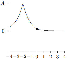
Figure 10.7:A wave packet on a stretched string, at .
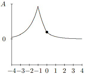
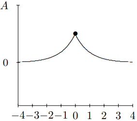
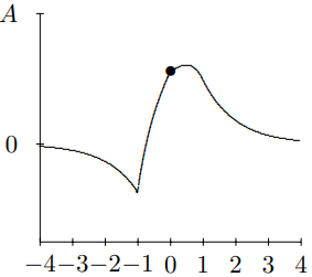
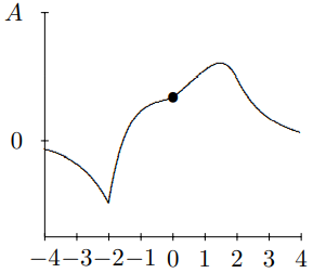
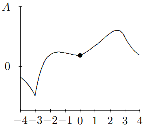
to 3. At , you see the pulse approaching the mass for negative . At , you can begin to see the effect of the mass on the string. By , the string to the left of is moving rapidly downwards. At , downward motion of the string for has continued, and has begun to form the reflected pulse. For , you can see the transmitted and reflected waves beginning to separate. For , you can see the reflected and transmitted pulses have separated almost completely and the mass has returned nearly to its equilibrium position. For large positive , the pulse is split into a reflected and transmitted wave.
The really interesting stuff is going on between and , so we will look at this on a finer time scale in . To really appreciate this, you should see it in motion. It is animated in program 10-4.
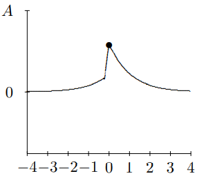
Figure 10.13:This is .
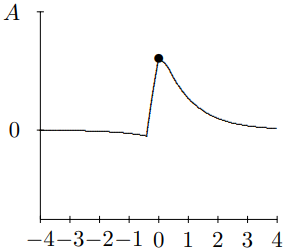
Figure 10.14:This is .
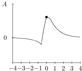
Figure 10.15:This is .
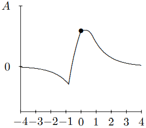
Figure 10.16:This is .
10.5: Is the Speed of Light?
We have seen that an electromagnetic wave in the direction satisfying Maxwell’s equations in free space has the dispersion relation 8.47, so that light, at least in vacuum, travels at the speed of light. But is the theory right? How do we test the dispersion relation? In fact, the most sensitive tests of Maxwell’s equations do not involve traveling waves. They come from observations of magnetic fields that extend over astrophysical distances (like the galaxy!). However, there is an interesting, if not very sensitive, way of looking for corrections to 8.47 that involves the speed of light directly. Before discussing this, let us digress briefly to talk in more detail about photons, the particles of light that we described briefly in chapter 8.
Light is a wave phenomenon, as we have seen. Indeed, the wave properties of light are obvious in our everyday experience. It is less obvious from our everyday experience, but equally true, that light also consists of photons. This becomes obvious when you work with light at very low intensities and/or very high energies. That both of these statements can be true simultaneously is one of the (many) miracles of quantum mechanics.
Quantum mechanics tells us that all particles have wave properties. A particle with momentum and energy has an associated angular frequency and angular wave number related by
where is Planck’s constant divided by . This combination appears so ubiquitously in quantum mechanics that it has its own symbol, and we physicists almost always use rather than . The reason is just that is related to the frequency rather than the angular frequency, , and we have seen that is the more convenient measure for most purposes. In addition, the energy and momentum of the particle are related as follows:
where is the rest mass and is the classical velocity.
If we put 10.105 into 10.106, we get a dispersion relation for the quantum mechanical wave associated with the particle
The classical velocity is the group velocity of the quantum mechanical wave!
In fact, particles, in a quantum mechanical picture, correspond to wave packets that move with the group velocity.
The quantum mechanical dispersion relation, 10.107, agrees with 8.47 only if . Thus we can restate the question of whether 8.47 is correct by asking “Is the photon mass really zero?”
It would seem that we ought to be able to test this idea by looking at two photons with different frequencies emitted at the same time from a far away object and checking whether they arrive at the same time. There is an obvious flaw in this scheme. If the object is so far away that we cannot get there, how do we know that the two photons were emitted at the same time? In fact, astrophysics has provided us with a way around this difficulty. We can look at pulsars. Pulsars are (presumably) rotating neutron star remnants of supernova explosions that emit light toward the earth at regular intervals. For example, pulsar 1937+21 is so regular that the departure time of photons can be determined to within a few microseconds ().[3] It is also about 16,000 light years away, so the photons with the higher frequency (the faster ones) have plenty of time to get ahead. When this experiment is done, one finds a nonzero , of about , corresponding to a mass of about . That seems like a rather small mass, but in fact, it is ridiculously large for a photon. From studies of the galactic magnetic field, we suspect that it is less than ![4] Thus something else is going on.
The problem with this measurement as a test of the dispersion relation is that there are electrons lying around out there — free electrons in interstellar space (10-1 to ). These electrons in space will wiggle in the field — this will produce a current density that will affect Maxwell’s equations, and that, in turn, will affect the dispersion relation. Let us analyze the effect of this dilute plasma assuming that the electron density is constant. Then (at least for the long wavelength radio waves of interest in these experiments) we can still use translation invariance to understand what is happening. Consider a plane wave in the direction and suppose that the electric field of the plane wave is in the direction. Then it is still true that at a given
for some . To find , we must look at the effect of the electric fields on the electrons, and then go back to Maxwell’s equations. The fields are very small, and for small fields the induced electron velocities, are small. Thus we can neglect . Then the force on an electron at the point is
The displacement of the electron has the same form:
which implies
comparing 10.110 and 10.112 gives
Thus the electrons are displaced out of phase with the electric field and in the same direction. Then the electron velocity is
The movement of the electrons gives rise to a current density:7
where is the electron number density.
Putting this into the relevant Maxwell’s equations, we find
or using , 8.47,
or solving for
The constant in (10.118) is called the “plasma frequency.” The amazing thing is that it looks just like a photon mass. For , this is consistent with the observation from the pulsar.
7Notice that the result is inversely proportional to the electron mass. This why we are concentrating on electrons rather than protons. The protons don’t move as fast!