Homework 6¶

Total points: 100

import numpy as np
from math import *
import matplotlib.pyplot as plt
import pandas as pd
%matplotlib inline
plt.style.use('seaborn-v0_8-colorblind')

Introduction to Homework 6¶

This homework’s exercises focus on oscillators and how to approximate the solution to the equations of motion using the SHO. The relevant reading background is:

chapter 5 of Taylor
chapter 6.6-6.8 of Boas
chapters 2.0-2.3 and 5.0-5.2 of Strogatz

In both textbooks there are many nice worked out examples.

Practicalities about homeworks and projects¶

You can work in groups (optimal groups are often 2-3 people) or by yourself. If you work as a group you can hand in one answer only if you wish. Remember to write your name(s)!
Homeworks are available ten days before the deadline.
Submission instructions: Submit the paper-and-pencil exercises as a single scanned PDF document. For this homework, this applies to exercises 1–5. Convert the Jupyter notebook to a PDF and attach it to the same PDF document.

Exercise 1 (10pt) Morse Potential as an SHO¶

If the potential has a local minimum, we can often find an SHO approximation for that potential near the local minimum.

The Morse potential is a convenient model for the potential energy of a diatomic molecule. The potential is a radial one and thus one-dimensional. It is given by,

U(r) = A\left[ \left(e^{(R-r)/S}-1\right)^2-1\right]

(1)

where the distance between the centers of the two atoms is $r$ , and the constants $A$ , $R$ , and $S$ are all positive. Here $S\ll R$ . Assume the moving coordinate has mass $m$ .

1a (2pt) Sketch (or plot) the potential as a function of $r$ .
1b (3pt) Find the equilibrium position of the potential, i.e. the position where the potential is at a minimum. We will call this $r_e$ .
1c (3pt) Rewrite the potential in terms of the displacement from equilibrium, $r = r_e + x$ . Expand the potential to second order in $x$ .
1d (2pt) Find the effective spring constant, $k$ , for the potential near the minimum. What is the frequency of small oscillations about the minimum?

Exercise 2 (10pt), Time Averaging and the SHO¶

Time averaging is a common tool for periodic systems. It allows us to discuss what happens to different properties of the system over one period.

An SHO has a period $\tau$ . We can find the time average of a variable $f(t)$ over one period, $\langle f \rangle$ , by averaging over the period,

\langle f \rangle = \frac{1}{\tau}\int_0^\tau f(t)dt

(2)

2a (2pt) Show that the time average of the position of the SHO is zero.
2b (2pt) Show that the time average of the velocity of the SHO is zero.
2c (6pt) Show that the time average of the kinetic energy of the SHO is equal to the time average of the potential energy (and importantly, non-zero). If the total energy is $E$ , these time averages are equal to $E/2$ . You might need to show that the very useful trigonometric identity,

\langle \sin^2(\omega t-\delta)\rangle = \langle \cos^2(\omega t-\delta)\rangle = \frac{1}{2}

(3)

Exercise 3 (10pt), Toy Potential¶

Consider a toy potential of the form,

U(r) = U_0\left(\dfrac{r}{R}+\lambda^2\frac{R}{r}\right)

(4)

where $U_0$ , $R$ , and $\lambda$ are all positive constants and the domain of the potential is $0<r<\infty$ .

3a (2pt) Sketch (or plot) the potential as a function of $r$ .
3b (3pt) Find the equilibrium position of the potential, i.e. the position where the potential is at a minimum. We will call this $r_e$ .
3c (5pt) Rewrite the potential in terms of the displacement from equilibrium, $r = r_e + x$ . Expand the potential to second order in $x$ . What is the effective spring constant, $k$ , for the potential near the minimum? What is the frequency of small oscillations about the minimum?

Exercise 4 (10pt), Defining Periodicity¶

A common issue with oscillators is determining their periodicity. For the SHO, we can show that the period is $2\pi/\omega_0$ where $\omega_0$ is the natural frequency of the SHO. How might we define a periodicity more generally? Let’s start with the damped harmonic oscillator. Consider a weakly damped oscillator ( $\beta < \omega_0$ ). The motion of the oscillator is given by,

x(t) = A e^{-\beta t}\cos(\omega_1 t - \delta)

(5)

where $A$ is the amplitude, $\beta$ is the damping constant, $\omega_1 = \sqrt{\omega_0^2 - \beta^2}$ and $\delta$ is the phase.

The motion decays with time, but we can still define a periodicity, $\tau_1$ , which is the time between peaks in the motion.

4a (4pt) Sketch (or plot) the motion of the oscillator as a function of time. Show that the oscillation period (the period of the underlying cosine factor) is $\tau_1 = 2\pi/\omega_1$ . Show that, despite the decaying envelope, successive same-type extrema (e.g., consecutive peaks) of $x(t)$ remain separated by exactly this interval -- this is why peak-to-peak timing gives an exact measurement of $\omega_1$ .
4b (3pt) Show that an equivalent definition of $\tau_1$ is twice the time between zero crossings of the motion.
4c (3pt) If the damping $\beta$ is half the natural frequency ( $\omega_0$ ), how does the amplitude of the motion decay in one period?

Exercise 5 (10pt), Planning your Final Project¶

The point of this exercise is to get you thinking about what you want to do for a final project and how you will accomplish it. Research and project planning are important skills to develop and it takes time to do so. We are trying to scaffold that development and give you the opportunity to practice these skills. So, you will be responsible for developing a plan for your final project, and the timeline under which you will accomplish it. Our job is to provide feedback and guidance on your plan, and to offer support in the development and construction of your final project.

Remember there is no right or wrong way to do this, it is about developing a plan that works for you.

Your final project is your chance to bring all the tools we have developed to bear on a question that interests you. You have reviewed the information on computational essays before, but here it is again in case it’s useful for this exercise:

Wolfram’s What is a Computational Essay?
The short paper Computational Essays: An Avenue for Scientific Creativity in Physics
Wolfram’s Steps to Writing a Computational Essay
University of Oslo’s Computational Essay Showroom

For your final project, you may work alone, in pairs, or in groups of up to three people. The expectation for your work will be higher if you have more people in your group; your explorations will need to be more comprehensive and detailed, and your essay will be expected to be longer and more polished if you have more people in your group. You can also develop more interesting ways of presenting your work that demonstrate the creativity and depth of your explorations if you have more people in your group. If you have any questions, just ask.

For this exercise, we want you to get started on planning your final project by sending us a brief proposal with a timeline. To help you, we have provided a schedule where you can see the checkpoints for your project, and when we will have a comprehensive work period. You should take advantage of that work period to make significant progress on your project; especially if there are technical aspects you are unsure about.

Project checkpoints¶

Plan regular project updates, a focused work period, and a final submission. The exact schedule can be set by the instructor or adapted for independent study.

Your Proposal¶

Your proposal should be a one to two page, single spaced, document that outlines the following:

The question you are interested in exploring. The motivation and interest to you and your group mates should be made clear. That is, motivate the question, why is it interesting?
References that provide background for this work. This should include the sites, resources, and references you have consulted to get started.
The approach you think you need to take to answer this question. Include the concepts and tools you plan to use to explore the question. That is, what have we developed in class that you will use to explore the question?
The timeline for your project. This should include the checkpoints in the schedule above, and any additional milestones you think are important. Consider making a Gantt chart to help you plan your project. This is a useful tool for planning and tracking your progress. It’s almost expected for proposals in science and engineering. Here, We suggest you take advantage of that work period to make significant progress on or to polish your project.

Your writing¶

You should consider this a formal proposal. It should be well written, clear, and concise. You should also consider the audience for this proposal. You should write this proposal for someone who is not in this class, but does know physics. Think about writing this to another student, a graduate student, or a professor. Someone that has a good understanding of physics, but not necessarily the details of your physics. You need to explain the motivation, the physics background, the approach, and the timeline in a way that is compelling and clear.

Your proposal need not be long, but it should be complete. Here are some additional resources for you to develop a good proposal:

Reference pages do not count towards the length, so if you have a lot of references, that’s fine. But the main text should be one to two pages. This is how it works with most proposals in science and engineering.

Exercise 6 (50 pt), Find your own 1D Oscillator¶

We have built all the tools to study 1D unforced oscillators. Now you get to pick your own potential and study it. You can pick any 1D potential you like, but it should have a local minimum. Make sure it is not a driven oscillator (i.e., no explicit time dependence in the equations of motion). To earn full credit for this exercise, you must:

6a (5pt) Present the potential and describe its origin, why it is interesting, where it comes from, etc. Educate us about it.
6b (5pt) Sketch (or plot) the potential as a function of its argument (and chosen variables) and find the equilibrium position of the potential, i.e. the position where the potential is at a minimum.
6c (10pt) Rewrite the potential in terms of the displacement from equilibrium. Expand the potential to second order to find the effective spring constant, $k$ , for the potential near the minimum. What is the frequency of small oscillations about the minimum?
6d (10pt) Construct the equations of motion for the potential and solve them numerically. Choose initial conditions and parameters that give oscillatory motion. It does not have to be an SHO; in fact, it probably will not be. Plot the position as a function of time. Make sure we can see the oscillations.
6e (10pt) Plot the phase diagram of the trajectory (you don’t have to produce a phase diagram, but just plot the trajectory in phase space). What does the phase diagram tell you about the motion?
6f (10pt) Find the period of your motion. Here you might have to make some definitions of what periodicity means for your potential.

Note: this might seem similar to your midterm, but notice we expect you to do some research on the potential in 6a, and we are going into more depth with questions 6e and 6f. This is also a scaffold for your final project in terms of practicing aspects that should appear.

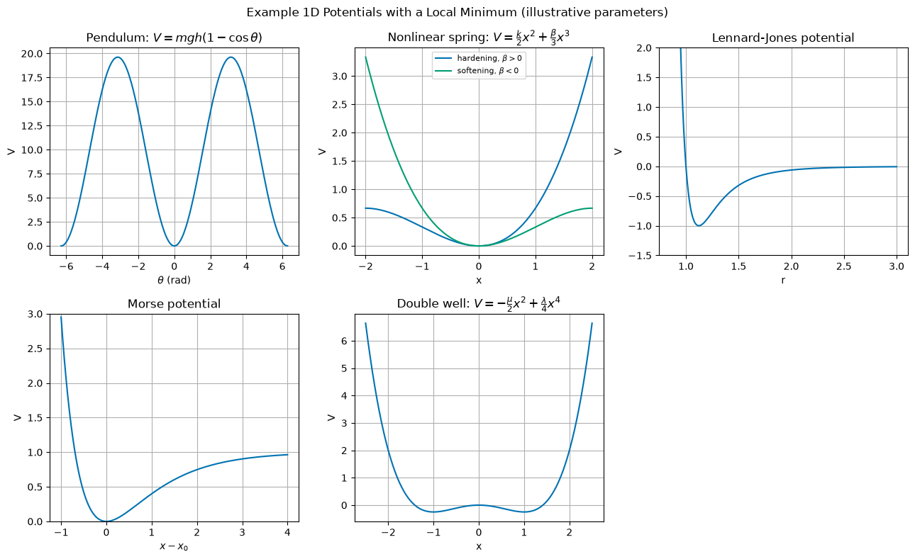
Examples of 1D potentials¶

Simple Pendulum (Nonlinear Small Angle Approximation)¶

V(\theta) = mgh(1 - \cos(\theta))

(6)

where $m$ is the mass, $g$ is the acceleration due to gravity, $h$ is the length of the pendulum, and $\theta$ is the angular displacement.

Nonlinear Spring (Hardening or Softening)¶

V(x) = \frac{k}{2} x^2 + \frac{\beta}{3} x^3

(7)

where $k$ and $\beta$ are constants. Depending on the sign of $\beta$ , the spring can exhibit hardening ( $\beta > 0$ ) or softening ( $\beta < 0$ ) nonlinearity.

Lennard-Jones Potential Oscillator (for a diatomic molecule model):¶

V(r) = 4\epsilon \left[ \left(\frac{\sigma}{r}\right)^{12} - \left(\frac{\sigma}{r}\right)^6 \right]

(8)

where $\epsilon$ is the depth of the potential well, $\sigma$ is the finite distance at which the inter-particle potential is zero, and $r$ is the distance between particles.

Morse Potential (for molecular vibrations)¶

V(x) = D_e \left(1 - e^{-a(x - x_0)}\right)^2

(9)

where $D_e$ is the depth of the potential well, $a$ is a constant related to the width of the well, $x$ is the displacement from equilibrium, and $x_0$ is the equilibrium bond length. This potential models the energy of a diatomic molecule as a function of the distance between atoms, showing oscillatory behavior that represents molecular vibrations.

Double Well Potential¶

V(x) = -\frac{\mu}{2} x^2 + \frac{\lambda}{4} x^4

(10)

where $\mu$ and $\lambda$ are positive constants. This system exhibits bistability with two stable equilibria, leading to interesting nonlinear dynamics and potential oscillations between the wells under certain conditions.

Each of the potentials above has a local minimum where the small-oscillation (SHO) approximation applies; the plots below use arbitrary illustrative parameter values, not a solution to any part of this problem.

import numpy as np
import matplotlib.pyplot as plt
plt.style.use('seaborn-v0_8-colorblind')

fig, axs = plt.subplots(2, 3, figsize=(13, 8))

# Simple pendulum
theta = np.linspace(-2*np.pi, 2*np.pi, 400)
m, g, h = 1.0, 9.81, 1.0
V = m*g*h*(1 - np.cos(theta))
axs[0, 0].plot(theta, V)
axs[0, 0].set_title('Pendulum: $V=mgh(1-\\cos\\theta)$')
axs[0, 0].set_xlabel(r'$\theta$ (rad)')
axs[0, 0].set_ylabel('V')

# Nonlinear spring (hardening vs softening)
x = np.linspace(-2, 2, 400)
k = 1.0
for beta, label in [(0.5, 'hardening, $\\beta>0$'), (-0.5, 'softening, $\\beta<0$')]:
    V = 0.5*k*x**2 + (beta/3)*x**3
    axs[0, 1].plot(x, V, label=label)
axs[0, 1].set_title(r'Nonlinear spring: $V=\frac{k}{2}x^2+\frac{\beta}{3}x^3$')
axs[0, 1].set_xlabel('x')
axs[0, 1].legend(fontsize=8)

# Lennard-Jones
r = np.linspace(0.85, 3, 400)
eps, sigma = 1.0, 1.0
V = 4*eps*((sigma/r)**12 - (sigma/r)**6)
axs[0, 2].plot(r, V)
axs[0, 2].set_ylim(-1.5, 2)
axs[0, 2].set_title('Lennard-Jones potential')
axs[0, 2].set_xlabel('r')

# Morse
x = np.linspace(-1, 4, 400)
De, a = 1.0, 1.0
V = De*(1 - np.exp(-a*x))**2
axs[1, 0].plot(x, V)
axs[1, 0].set_ylim(0, 3)
axs[1, 0].set_title('Morse potential')
axs[1, 0].set_xlabel(r'$x-x_0$')

# Double well
x = np.linspace(-2.5, 2.5, 400)
mu, lam = 1.0, 1.0
V = -0.5*mu*x**2 + 0.25*lam*x**4
axs[1, 1].plot(x, V)
axs[1, 1].set_title(r'Double well: $V=-\frac{\mu}{2}x^2+\frac{\lambda}{4}x^4$')
axs[1, 1].set_xlabel('x')

axs[1, 2].axis('off')

for ax in axs.flat:
    if ax.axison:
        ax.set_ylabel('V')
        ax.grid(True)

fig.suptitle('Example 1D Potentials with a Local Minimum (illustrative parameters)')
plt.tight_layout()
plt.show()