Homework 3¶

Total points: 100.

Introduction to homework 3¶

This homework’s sets of classical pen and paper and computational exercises deal with the motion of different objects under the influence of various forces. The relevant reading background is

1. chapter 2 of Taylor (there are many good examples there)

2. chapters 5-7 of Malthe-Sørenssen.

In both textbooks there are many nice worked out examples. Malthe-Sørenssen’s text contains also several coding examples you may find useful.

There are several pedagogical aims we have in mind with these exercises:

1. Get practice in setting up and analyzing a physical problem, finding the forces and the relevant equations to solve;

2. Analyze the results and ask yourself whether they make sense or not;

3. Find analytical solutions to problems when possible and compare them with numerical results. This also teaches us how to understand errors in numerical calculations;

4. Being able to solve (in mechanics these are the most common types of equations) numerically ordinary differential equations and compare the solutions where possible with analytical solutions;

5. Getting used to studying physical problems using all possible tools, from paper and pencil to numerical solutions;

6. Analyze the results and ask yourself whether they make sense.

The above steps outline important elements of our understanding of the scientific method. Furthermore, there are also explicit coding skills we aim at such as setting up arrays, solving differential equations numerically and plotting your results. Coding practice is also an important aspect. The more we practice the better we get (hopefully). From a numerical mathematics point of view, we will solve the differential equations using Euler’s method (forward Euler).

The code we will develop can be reused as a basis for coming homeworks. We can also extend the numerical solver we write here to include other methods (later) like the modified Euler method (Euler-Cromer, midpoint Euler) and more advanced methods like the family of Runge-Kutta methods and the Velocity-Verlet method.

At the end of this course, we will thus have developed a larger code (or set of codes) which will allow us to study different numerical methods (integration and differential equations) as well as being able to study different physical systems. Combined with analytical skills, the hope is that this can allow us to explore interesting and realistic physics problems. By doing so, the hope is that can lead to deeper insights about the laws of motion which govern a system.

And hopefully you can reuse many of the above solvers in other courses (our ideal).

Practicalities about homeworks and projects¶

1. You can work in groups (optimal groups are often 2-3 people) or by yourself. If you work as a group you can hand in one answer only if you wish. Remember to write your name(s)!

2. Homeworks are available ten days before the deadline.

3. Submission instructions: Submit the paper-and-pencil exercises as a single scanned PDF document. For this homework, this applies to exercises 1–5. Convert the Jupyter notebook to a PDF and attach it to the same PDF document.

Exercise 1 (20 pt), Electron moving into an electric field¶

An electron is sent through a varying electrical field. Initially, the electron is moving in the $x$-direction with a velocity $v_x = 100$ m/s. The electron enters the field when it passes the origin. The field varies with time, causing an acceleration of the electron that varies in time

• 1a (4pt) Find the velocity as a function of time for the electron.

• 1b (4pt) Find the position as a function of time for the electron.

The field is only acting inside a box of length $L = 2m$.

• 1c (4pt) For how long time is the electron inside the field?

• 1d (4pt) What is the displacement in the $y$-direction when the electron leaves the box. (We call this the deflection of the electron).

• 1e (4pt) Find the angle the velocity vector forms with the horizontal axis as the electron leaves the box.

Exercise 2 (10 pt), Drag force¶

We can observe that the models for linear and quadratic drag forces are given by:

where $D$ is the “length scale” of the object (e.g., the diameter of the sphere), $\eta$ is the viscosity of the fluid, $\rho$ is the density of the fluid, $A$ is the cross-sectional area of the object, and $\kappa$ is a constant of order unity (larger for flat and blunt bodies; smaller for streamlined bodies).

The two force laws scale differently with speed, as illustrated below for arbitrary parameter values.

import numpy as np
import matplotlib.pyplot as plt
plt.style.use('seaborn-v0_8-colorblind')

v = np.linspace(0, 5, 200)
D = 0.5  # illustrative length scale [m]
eta = 1.8e-5  # air viscosity [Pa s]
rho = 1.2  # air density [kg/m^3]
kappa = 0.25
A = np.pi * (D / 2) ** 2

f_lin = 3 * np.pi * eta * D * v
f_quad = kappa * rho * A * v ** 2

fig, ax = plt.subplots(figsize=(6, 4.5))
ax.plot(v, f_lin, label='Linear drag, $f_{lin} = 3\\pi \\eta D v$')
ax.plot(v, f_quad, label='Quadratic drag, $f_{quad} = \\kappa \\rho A v^2$')
ax.set_xlabel('Speed $v$ (m/s)')
ax.set_ylabel('Drag force (N)')
ax.set_title('Linear vs. Quadratic Drag Force (illustrative)')
ax.legend()
ax.grid(True)
plt.tight_layout()
plt.show()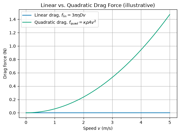

• 2a (5pt) The Reynolds number is defined as $Re = \rho v D / \eta$. What is the physical meaning of this number? For a spherical object, show that the ratio of the quadratic drag force to the linear drag force is given by $f_{quad}/f_{lin} = Re/48$. Use this to explain the physical meaning of the Reynolds number. Note: you may assume that $\kappa = 0.25$ for a sphere.

• 2b (2pt) Explain a situation where there would be a low Reynolds number. What about a high Reynolds number? Estimate the Reynolds number for a falling rain drop, a parachutist, a car, and a plane.

• 2c (3pt) Find another dimensionless number from fluid mechanics and explain its physical meaning. Make sure you consider high and low values of the number you find.

Exercise 3 (10 pt), Falling object¶

We have shown that an object that is dropped from rest and experiences linear drag force will reach a terminal velocity and do so exponentially:

• 3a (4pt) At first, the object will be moving slowly. Show that we can approximate this expression in that interval. We should find that $v_y = gt$ -- the standard result for free fall in vacuum. Demonstrate this.

• 3b (3pt) What is the next term, $O(t^2)$, in the expansion? What is the physical meaning of this term?

• 3c (4pt) The position of the object, measured positive downward, is given by: $y(t) = v_{ter}t + (v_{y0}-v_{ter})\tau(1-e^{-t/\tau})$. Show that this reduces to the standard result $y = \frac{1}{2}gt^2$ when $v_{y0} = 0$. What is the small parameter in your expansions in all cases?

Exercise 4 (10 pt), and now a theoretical exercise¶

Finding and exploring equations of motion is the central enterprise of classical mechanics. You will encounter (and derive) many equations you have not seen before, and you will need to explain them. Consider a hypothetical one-dimensional system where a mass $m$ has a speed of $v_0$ and coasts along the x-axis. The surrounding medium produces a drag force that is modeled using:

When the force is a pure function of velocity, using the technique called separation of variables on Newton’s 2nd Law, we can find the velocity as a function of time:

We can separate variables and write:

Divide both sides by $F(v)$ and multiply both sides by $dt$:

And then, given starting (initial) conditions, we integrate both sides to find an expression for $t$ as a function of $v$.

• 4a (4pt) For the given force above, write the equation of motion in a form: $\dfrac{m dv}{F(v)} = dt$. Integrate both sides to find an expression for the velocity $v$ as a function of $t$ ($v(t)$ not $t(v)$).

• 4b (2pt) Check your answer by looking at the limits of its behavior. Does it agree with your intuition?

• 4c (2pt) Sketch the expression and explain what the motion of the object looks like by interpreting this expression and your sketch.

• 4d (2pt) Will the object ever come to rest?

Exercise 5 (10 pt), back to a falling ball and preparing for the numerical exercise¶

Useful material: Malthe-Sørenssen chapter 7.5 and Taylor chapter 2.4.

In this example we study the motion of an object subject to a constant force and a velocity dependent force. We will reuse the code we develop here in homework 4 for a position-dependent force.

Here we limit ourselves to a ball that is thrown from a height $h$ above the ground with an initial velocity $\vec{v}_0$ at time $t=t_0$. We assume the air resistance is proportional to the square velocity. Together with the gravitational force these are the forces acting on our system.

In order to find an analytical solution we need to assume that the object is falling only in the $y$-direction, with downward chosen as positive for this one-dimensional subproblem.

The position of the ball as function of time is $\vec{r}(t)$ where $t$ is time. The position is measured with respect to a coordinate system with origin at the floor.

We assume we have an initial position $\vec{r}(t_0)=h\vec{e}_y$ and an initial velocity $\vec{v}_0=v_{x,0}\vec{e}_x+v_{y,0}\vec{e}_y$.

In this exercise we assume the system is influenced by the gravitational force

and an air resistance given by a square law

The analytical expressions for velocity and position as functions of time will be used to compare with the numerical results in exercise 6.

• 5a (3pt) Identify the forces acting on the ball and set up a diagram with the forces acting on the ball. Find the equation of motion for the falling ball. Do not limit to 1D yet!

• 5b (4pt) Assume now that the object is falling only in the $y$-direction and take downward as positive for this subproblem. Integrate the equation of motion from an initial time $t_0$ to a final time $t$ and find the velocity. Assume it is dropped from rest to simplify the mathematics. In Taylor equations (2.52) to (2.58) you will find a very good discussion of this.

• 5c (3pt) Find thereafter the position as function of time starting with an initial time $t_0$. Find the time it takes to hit the floor. Here you will find it convenient to set the initial velocity in the $y$-direction to zero. Taylor equations (2.52)-(2.58) should contain all relevant information for solving this part as well.

We will use the above analytical results in our numerical calculations in exercise 6. The analytical solution in the $y$-direction only will serve as a test for our numerical solution. We don’t often know the solutions to our problems exactly, so we have to check them against things we do know.

Exercise 6 (40pt), Numerical elements, solving exercise 5 numerically¶

This exercise should be handed in as a jupyter-notebook through the course submission system. Remember to write your name(s).

Previously, we:

1. Gained more practice with plotting in Python

2. Became familiar with arrays and representing vectors with such objects

In this homework, we will:

1. Learn and utilize Euler’s Method to find the position and the velocity

2. Compare analytical and computational solutions

3. Add additional forces to our model

%matplotlib inline

# let's start by importing useful packages we are familiar with
import numpy as np
import matplotlib.pyplot as plt
%matplotlib inline

We will choose the following values

1. mass $m=0.2$ kg

2. acceleration (gravity) $g=9.81$ m/s$^{2}$.

3. initial position is the height $h=2$ m

4. initial velocities $v_{x,0}=v_{y,0}=10$ m/s

Can you find a reasonable value for the drag coefficient $D$? You need also to define an initial time and the step size $\Delta t$. We can define the step size $\Delta t$ as the difference between any two neighboring values in time (time steps) that we analyze within some range. It can be determined by dividing the interval we are analyzing, which in our case is time $t_{\mathrm{final}}-t_0$, by the number of steps we are taking $(N)$. This gives us a step size $\Delta t = \dfrac{t_{\mathrm{final}}-t_0}{N}$.

With these preliminaries we are now ready to plot our results from exercise 5.

• 6a (10pt) Set up arrays for time, velocity, acceleration and positions for the results from exercise 5. Define an initial and final time. Choose the final time to be the time when the ball hits the ground for the first time. Make a plot of the position and velocity as functions of time. Here you could set the initial velocity in the $y$-direction to zero and use the result from exercise 5. Else you need to try different initial times using the result from exercise 5 as a starting guess. It is not critical if you don’t reach the ground when the initial velocity in the $y$-direction is not zero.

We move now to the numerical solution of the differential equations as discussed in the lecture notes or Malthe-Sørenssen chapter 7.5. Let us remind ourselves about Euler’s Method.

Suppose we know $f(t)$ and its derivative $f'(t)$. To find $f(t+\Delta t)$ at the next step, $t+\Delta t$, we can consider the Taylor expansion:

$f(t+\Delta t) = f(t) + \dfrac{(\Delta t)f'(t)}{1!} + \dfrac{(\Delta t)^2f''(t)}{2!} + ...$

If we ignore the $f''$ term and higher derivatives, we obtain

$f(t+\Delta t) \approx f(t) + (\Delta t)f'(t)$.

This approximation is the basis of Euler’s method, and the Taylor expansion shows that the local truncation error is $O(\Delta t^2)$, while the global error over a fixed interval is generally $O(\Delta t)$. Thus, one would expect it to work better, the smaller the step size $h$ that you use. In our case the step size is $\Delta t$.

In setting up our code we need to

1. Define and obtain all initial values, constants, and time to be analyzed with step sizes as done above (you can use the same values)

2. Calculate the velocity using $v_{i+1} = v_{i} + (\Delta t)*a_{i}$

3. Calculate the position using $pos_{i+1} = r_{i} + (\Delta t)*v_{i}$

4. Calculate the new acceleration $a_{i+1}$.

5. Repeat steps 2-4 for all time steps within a loop.

• 6b (20 pt) Write a code which implements Euler’s method and compute numerically and plot the position and velocity as functions of time for various values of $\Delta t$. Comment your results.

• 6c (10pt) Compare your numerically obtained positions and velocities with the analytical results from exercise 5. In order to do this, you need to take out the motion in the $x$-direction. Comment again your results.