Total points: 100.
Practicalities about homeworks and projects
You can work in groups (optimal groups are often 2-3 people) or by yourself. If you work as a group you can hand in one answer only if you wish. Remember to write your name(s)!
Homeworks are available approximately ten days before the deadline. You should anticipate this work.
Submission instructions: Submit the paper-and-pencil exercises as a single scanned PDF document. For this homework, this applies to exercises 1–5. Convert the Jupyter notebook to a PDF and attach it to the same PDF document.
Exercise 1 (10 pt), Forces, discussion questions, test your intuition
These questions expect not only an answer, but an explanation of your reasoning.
To receive full credit, these answers should include both the underlying physics that explains your answer and a reflection on your reasoning (for example, whether you are confident in the answer). Physics intuition develops over time and often needs to be reconciled with everyday experience.
1a (2pt) Single force. Can an object affected only by a single force have zero acceleration?
1b (2pt) Zero velocity. If you throw a ball vertically it has zero velocity at its maximum point. Does it also have zero acceleration at this point?
1c (3pt) Acceleration due to gravity. You measure the acceleration of gravity in an elevator moving downward at a constant velocity of . What will you measure?
1d (3pt) Air resistance. You throw a ball straight up and measure the velocity as it passes you on its way down. Will the velocity be larger, the same, or smaller if you did the same experiment in vacuum?
Exercise 2 (10 pt), setting up forces, Newton’s second law
Useful material here to read is
Taylor chapters 1.3 and 1.4
Malthe-Sørenssen chapters 5.1, 5.2 and 5.3
A person jumps from an airplane, falling freely for several seconds before the person pulls the cord of the parachute and the parachute unfolds.
2a (3pt) Identify the forces acting on the parachutist and draw a free-body diagram of the parachutist before the person has pulled the cord. Include a brief discussion of any assumptions you make, motivate and justify your choices.
2b (3pt) Identify the forces acting on the parachutist and draw a free-body diagram of the parachutist after the person has pulled the cord. Include a brief discussion of any assumptions you make, motivate and justify your choices.
2c (4pt) Sketch the net force acting on the parachutist as a function of time, . Choose and state a positive direction. Model the parachute deployment as a short transition from the pre-deployment drag force to the post-deployment drag force, and indicate the forces before and after deployment.
Exercise 3 (10 pt), Space shuttle immediately after lift-off
Useful material here to read is: Malthe-Sørenssen chapters 5.1, 5.2 and 5.3
During lift-off of the space shuttle, the engines provide an upward force of . The mass of the shuttle is approximately . Take upward as positive. Immediately after lift-off, the shuttle’s speed is approximately zero, so air resistance can be neglected at that instant.
3a (3pt) Draw a free-body diagram of the space shuttle immediately after lift-off.
3b (3pt) Find an expression for the acceleration of the space shuttle immediately after lift-off.
Let us assume that the force from the engines is constant and that the mass of the space shuttle does not change significantly over the first 20 s. Continue to ignore air resistance for this calculation.
3c (4pt) Find the velocity and position of the space shuttle after 20 s if you ignore air resistance.
Exercise 4 (15 pt), Hitting a golf ball
Useful material here to read is
Taylor chapters 1.3-1.6
Malthe-Sørenssen chapter 6.3-6.4 and 7.1-7.3
Do Taylor exercise 1.35. The formulae you obtain here will be useful for the numerical exercises below (see exercise 6 below).
Repeated below consistent with fair use practices
A golf ball is hit from ground level with a speed in a direction due east that is at an angle above the horizontal.
4a (5 pt) Neglecting air resistance, use Newton’s second law to find the position as a function of time, using the coordinates measured east, measured north, and measured up.
4b (5 pt) Find the time the golf ball is in the air and how far it travels in that time.
Reflect on the form of your answer.
4c (5 pt) Your answers should depend on and . What can you say about the dependence of the time the golf ball is in the air and the distance it travels on these two variables? How can we believe this functional form of your answer? How can we check it? Propose a check and check that your answer is consistent with this check.
Exercise 5 (15 pt), ball thrown along a sloped ramp
Taylor exercise 1.39. Make sure to draw your setup clearly, show your free-body diagram, and explain any assumptions you make to solve the problem.
Repeated below consistent with fair use practices
A ball is thrown with initial speed up an inclined plane. The plane is inclined at an angle above the horizontal, and the ball’s initial velocity is at an angle above the plane. Choose axes with measured up the slope, normal to the slope, and across it.
5a (5 pt) Write down Newton’s second law using these axes and find the ball’s position as a function of time. Make sure to include the FBD and any assumptions you make.
5b (5 pt) Show that the ball lands a distance
from its launch point. This is measured up the ramp (i.e., along it).
5c (5 pt) Show that for given and , the maximum range up the inclined plane is:
Exercise 6 (40pt), Numerical elements, moving to more than one dimension
This exercise should be handed in as a jupyter-notebook through the course submission system. Remember to write your name(s).
Previously, we:
Analytically mapped 1D motion over some time
Gained practice with functions
Reviewed vectors and matrices in Python
In this homework, we will:
Practice using Python syntax and variable manipulation
Utilize analytical solutions to create more refined functions
Work in two, three or even higher dimensions
This material will then serve as background for the numerical part of homework 3. The first part is a simple warm-up, with hints and suggestions you can use for the code to write below.
%matplotlib inline

# As usual, here are some useful packages we will be using. Feel free to use more and experiment as you wish.

import numpy as np
import matplotlib.pyplot as plt
from mpl_toolkits import mplot3d
%matplotlib inline
In class (the falling baseball example) we used an analytical expression for the height of a falling ball. In the first homework we used instead the position from experiment (Usain Bolt’s 100m record run) and stored this information with one-dimensional arrays in Python.
Let us get some practice with this. The cell below creates two arrays, one containing the times to be analyzed and the other containing the and components of the position vector at each point in time. This is a two-dimensional object. The second array is initially empty. Then we define the initial position to be and . Take a look at the code and comments to get an understanding of what is happening. Feel free to play around with it.
tf = 4 #length of value to be analyzed
dt = .001 # step sizes
t = np.arange(0.0,tf,dt) # Creates an evenly spaced time array going from 0 to 3.999, with step sizes .001
p = np.zeros((len(t), 2)) # Creates an empty array of [x,y] arrays (our vectors). Array size is same as the one for time.
p[0] = [2.0,1.0] # This sets the initial position to be x = 2 and y = 1
Below we are printing specific values of our array to see what is being stored where. The first number in the array represents which array iteration we are looking at, while the number after the represents which listed number in the array iteration we are getting back.
print(p[0]) # Prints the first array
print(p[0,:]) # Same as above, these commands are interchangeable
[2. 1.]
[2. 1.]
print(p[3999]) # Prints the 4000th array[0. 0.]
print(p[0,0]) # Prints the first value of the first array2.0
print(p[0,1]) # Prints the second value of first array
print(p[:,0]) # Prints the first value of all the arrays
1.0
[2. 0. 0. ... 0. 0. 0.]
Then try running this cell. Notice how it gives an error since we did not implement a third dimension into our arrays
#print(p[:,2])In the cell below we want to manipulate the arrays. In this example we make each vector’s component valued the same as their respective vector’s position in the iteration and the value will be twice that value, except for the first vector, which we have already set. That is we have
Here we set up an array for and values.
for i in range(1, len(p)):
    p[i] = [i,2*i]
# Checker cell to make sure your code is performing correctly
c = 0
for i in range(len(p)):
    if i == 0:
        if p[i,0] != 2.0:
            c += 1
        if p[i,1] != 1.0:
            c += 1
    else:
        if p[i,0] != 1.0*i:
            c += 1
        if p[i,1] != 2.0*i:
            c += 1

if c == 0:
    print("Success!")
else:
    print("There is an error in your code")
Success!
You could also think of an alternative way of storing the above information. Feel free to explore how to store multidimensional objects.
In the previous homework we studied Usain Bolt’s 100m run and in class we studied a falling baseball. We made basic plots of the baseball moving in one dimension. Now we will be working with a three-dimensional variant. This will be useful for our next homeworks and numerical projects.
Assume we have a soccer ball moving in three dimensions with the following trajectory:
Now let us create a three-dimensional (3D) plot using these equations. In the cell below we write the equations into their respective labels. We fix a final time in the code below.
Important Concept: Numpy comes with many mathematical packages, some of them being the trigonometric functions sine, cosine, tangent. We are going to utilize these here. Additionally, these functions work with radians, so we will also be using a function from Numpy that converts degrees to radians.
tf = 2.04  # The final time to be evaluated
dt = 0.1  # The time step size
t = np.arange(0,tf,dt) # The time array
theta_deg = 45 # Degrees
theta_rad = np.radians(theta_deg) # Converts degrees to their radian counterparts
x = 10*t*np.cos(theta_rad) # Equation for our x component, utilizing np.cos() and our calculated radians
y = 10*t*np.sin(theta_rad) # Put the y equation here
z = 10*t-9.81/2*t**2# Put the z equation here
Then we plot it
## Once you have entered the proper equations in the cell above, run this cell to plot in 3D
fig = plt.axes(projection='3d')
fig.set_xlabel('x')
fig.set_ylabel('y')
fig.set_zlabel('z')
fig.scatter(x,y,z)
<mpl_toolkits.mplot3d.art3d.Path3DCollection at 0x7f24b729b740>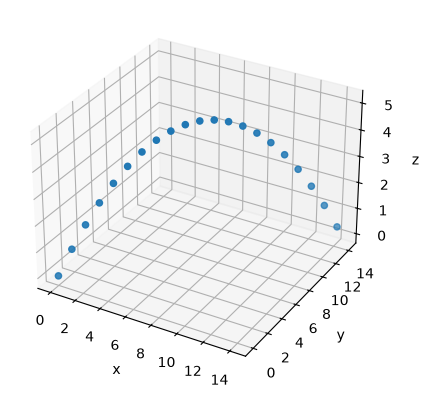
6a (8pt) How would you express , , for this problem as a single vector, ?
Define the position vector as r = np.array([x, y, z]), then run the code and plot using the array .
## Run this code to plot using our r array
# fig = plt.axes(projection='3d')
# fig.set_xlabel('x')
# fig.set_ylabel('y')
# fig.set_zlabel('z')
r = np.array([x, y, z])
fig.scatter(r[0],r[1],r[2])
<mpl_toolkits.mplot3d.art3d.Path3DCollection at 0x7f24b4fd9430>6b (8pt) What do you think the benefits and/or disadvantages are of expressing our three equations as a single array/vector? Discuss both computational and physical considerations. Use NumPy to print the maximum values of the , , and coordinates along the trajectory.
Complete Exercise 4 above (Taylor exercise 1.35) before moving further. (Recall that the golf ball was hit due east at an angle with respect to the horizontal, and the coordinate directions are measured east, north, and vertically up.)
6c (8pt) What is the analytical solution for our theoretical golf ball’s position over time from Exercise 4? Also find the time when the golf ball hits the ground. Use these results to develop a function, called
Golfballfor example, that takes an initial speed and the launch angle in degrees, produces a 3D graph of the motion, and finds the maximum values of , , and along the trajectory. State clearly how you determine each maximum.6d (8pt) Given initial values of , , what would our maximum x, y and z components be?
6e (8pt) Given initial values of , , what would our maximum x, y and z components be?