6.2 Numerical Methods in Trigonometry

We were able to solve the trigonometric equations in the previous section fairly easily, which in general is not the case. For example, consider the equation

There is a solution, as shown in Figure 6.2.1 below. The graphs of \(y=\cos\;x\) and \(y=x\) intersect somewhere between \(x=0\) and \(x=1\), which means that there is an \(x\) in the interval \(\ival{0}{1}\) such that \(\cos\;x = x\).

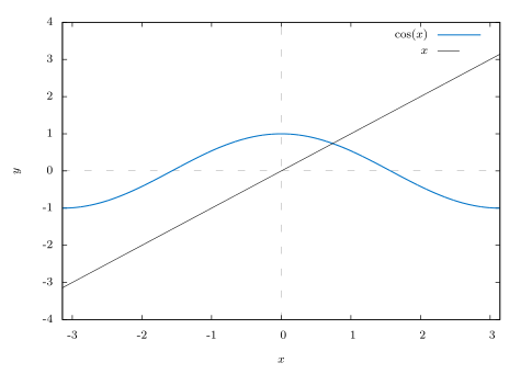
Unfortunately there is no trigonometric identity or simple method which will help us here. Instead, we have to resort to numerical methods, which provide ways of getting successively better approximations to the actual solution(s) to within any desired degree of accuracy. There is a large field of mathematics devoted to this subject called numerical analysis. Many of the methods require calculus, but luckily there is a method which we can use that requires just basic algebra. It is called the secant method, and it finds roots of a given function \(f(x)\), i.e. values of \(x\) such that \(f(x)=0\). A derivation of the secant method is beyond the scope of this book,^[1] but we can state the algorithm it uses to solve \(f(x)=0\):

1. Pick initial points \(x_0\) and \(x_1\) such that \(x_0 < x_1\) and \(f(x_0)\,f(x_1) < 0\) (i.e. the solution is somewhere between \(x_0\) and \(x_1\)).

2. For \(n \ge 2\), define the number \(x_n\) by

   \begin{equation} x_n ~=~ x_{n-1} ~-~ \dfrac{(x_{n-1} \;-\; x_{n-2})\,f(x_{n-1})}{f(x_{n-1}) \;-\; f(x_{n-2})} \tag{6.2}\end{equation}

   as long as \(\abs{x_{n-1} \;-\; x_{n-2}} > \epsilon_{error}\), where \(\epsilon_{error} > 0\) is the maximum amount of error desired (usually a very small number).

3. The numbers \(x_0\), \(x_1\), \(x_2\), \(x_3\), \(...\) will approach the solution \(x\) as we go through more iterations, getting as close as desired.

We will now show how to use this algorithm to solve the equation \(\cos\;x = x\). The solution to that equation is the root of the function \(f(x) =\cos\;x - x\). And we saw that the solution is somewhere in the interval \(\ival{0}{1}\). So pick \(x_0 = 0\) and \(x_1 = 1\). Then \(f(0)=1\) and \(f(1)=-0.4597\), so that \(f(x_0)\,f(x_1) < 0\) (we are using radians, of course). Then by definition,

and so on. Using a calculator is not very efficient and will lead to rounding errors. A better way to implement the algorithm is with a computer. Listing 1 below shows the code (secant.java) for solving \(\cos\;x = x\) with the secant method, using the Java programming language:

import java.math.*;
public class secant {
 public static void main (String[] args) {
   double x0 =  Double.parseDouble(args[0]);
   double x1 =  Double.parseDouble(args[1]);
   double x = 0;
   double error = 1.0E-50;
   for (int i=2; i <= 10; i++) {
      if (Double.compare(Math.abs(x0 - x1),error) > 0) {
         x = x1 - (x1 - x0)*f(x1)/(f(x1) - f(x0));
         x0 = x1;
         x1 = x;
         System.out.println("x" + i + " = " + x);
      } else {
         break;
      }
   }
   MathContext mc = new MathContext(50);
   BigDecimal answer = new BigDecimal(x,mc);
   System.out.println("x = " + answer);
 }
//Define the function f(x)
 public static double f (double x) {
   return Math.cos(x) - x;
 }
}

Lines 4-5 read in \(x_0\) and \(x_1\) as input parameters to the program.

Line 6 initializes the variable that will eventually hold the solution.

Line 7 sets the maximum error \(\epsilon_{error}\) to be \(1.0 \,\times\, 10^{-50}\). That is, our final answer will be within that (tiny!) amount of the real solution.

Line 8 starts a loop of 9 iterations of the algorithm, i.e. it will create the successive approximations \(x_2\), \(x_3\), \(...\), \(x_{10}\) to the real solution, though in Line 9 we check to see if the two previous approximations differ by less than the maximum error. If they do, we stop (since this means we have an acceptable solution), otherwise we continue.

Line 10 is the main step in the algorithm, creating \(x_n\) from \(x_{n-1}\) and \(x_{n-2}\).

Lines 11-12 set the new values of \(x_{n-2}\) and \(x_{n-1}\), respectively.

Lines 18-20 set the number of decimal places to show in the final answer to 50 (the default is 16) and then print the answer.

Lines 23-24 give the definition of the function \(f(x)=\cos\;x - x\). Below is the result of compiling and running the program using \(x_0 = 0\) and \(x_1 = 1\):

javac secant.java
java secant 0 1
x2 = 0.6850733573260451
x3 = 0.736298997613654
x4 = 0.7391193619116293
x5 = 0.7390851121274639
x6 = 0.7390851332150012
x7 = 0.7390851332151607
x8 = 0.7390851332151607
x = 0.73908513321516067229310920083662495017051696777344

Notice that the program only got up to \(x_8\), not \(x_{10}\). The reason is that the difference between \(x_8\) and \(x_7\) was small enough (less than \(\epsilon_{error} = 1.0 \,\times\, 10^{-50}\)) to stop at \(x_8\) and call that our solution. The last line shows that solution to 50 decimal places.

Does that number look familiar? It should, since it is the answer to Exercise 11 in Section 4.1. That is, when taking repeated cosines starting with any number (in radians), you eventually start getting the above number repeatedly after enough iterations. This turns out not to be a coincidence. Figure 6.2.2 gives an idea of why.

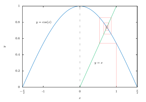
Since \(x=0.73908513321516...\) is the solution of \(\cos\;x = x\), you would get \(\cos\;(\cos\;x) = \cos\;x = x\), so \(\cos\;(\cos\;(\cos\;x)) = \cos\;x = x\), and so on. This number \(x\) is called an attractive fixed point of the function \(\cos\;x\). No matter where you start, you end up getting “drawn” to it. Figure 6.2.2 shows what happens when starting at \(x=0\): taking the cosine of \(0\) takes you to \(1\), and then successive cosines (indicated by the intersections of the vertical lines with the cosine curve) eventually “spiral” in a rectangular fashion to the fixed point (i.e. the solution), which is the intersection of \(y=\cos\;x\) and \(y=x\).

Recall in Example 5.10 in Section 5.2 that we claimed that the maximum and minimum of the function \(y=\cos\;6x + \sin\;4x\) were \(\pm\,1.90596111871578\), respectively. We can show this by using the open-source program Octave.^[2] Octave uses a successive quadratic programming method to find the minimum of a function \(f(x)\). Finding the maximum of \(f(x)\) is the same as finding the minimum of \(-f(x)\) then multiplying by \(-1\) (why?). Below we show the commands to run at the Octave command prompt (octave:n>) to find the minimum of \(f(x) = \cos\;6x + \sin\;4x\). The command sqp(3,’f’) says to use \(x=3\) as a first approximation of the number \(x\) where \(f(x)\) is a minimum.

octave:1> format long
octave:2> function y = f(x)
> y = cos(6*x) + sin(4*x)
> endfunction
octave:3> sqp(3,'f')
y = -1.90596111871578
ans = 2.65792064609274

The output says that the minimum occurs when \(x=2.65792064609274\) and that the minimum is \(-1.90596111871578\). To find the maximum of \(f(x)\), we find the minimum of \(-f(x)\) and then take its negative. The command sqp(2,’f’) says to use \(x=2\) as a first approximation of the number \(x\) where \(f(x)\) is a maximum.

octave:4> function y = f(x)
> y = -cos(6*x) - sin(4*x)
> endfunction
octave:5> sqp(2,'f')
y = -1.90596111871578
ans = 2.05446832062993

The output says that the maximum occurs when \(x=2.05446832062993\) and that the maximum is \(-(-1.90596111871578) = 1.90596111871578\).

Recall from Section 2.4 that Heron’s formula is adequate for “typical” triangles, but will often have a problem when used in a calculator with, say, a triangle with two sides whose sum is barely larger than the third side. However, you can get around this problem by using computer software capable of handling numbers with a high degree of precision. Most modern computer programming languages have this capability. For example, in the Python programming language^[3] (chosen here for simplicity) the decimal module can be used to set any level of precision.^[4] Below we show how to get accuracy up to \(50\) decimal places using Heron’s formula for the triangle in Example 2.16 from Section 2.4, by using the python interactive command shell:

>>> from decimal import *
>>> getcontext().prec = 50
>>> a = Decimal("1000000")
>>> b = Decimal("999999.9999979")
>>> c = Decimal("0.0000029")
>>> s = (a+b+c)/2
>>> K = s*(s-a)*(s-b)*(s-c)
>>> print Decimal(K).sqrt()
0.99999999999894999999999894874999999889618749999829

(Note: The triple arrow >>> is just a command prompt, not part of the code.)
Notice in this case that we do get the correct answer; the high level of precision eliminates the rounding errors shown by many calculators when using Heron’s formula.

Another software option is Sage^[5], a powerful and free open-source mathematics package based on Python. It can be run on your own computer, but it can also be run through a web interface: go to http://sagenb.org to create a free account, then once you register and sign in, click the New Worksheet link to start entering commands. For example, to find the solution to \(\cos\;x = x\) in the interval \(\ival{0}{1}\), enter these commands in the worksheet textfield:

x = var('x')
find_root(cos(x) == x, 0,1)

Click the evaluate link to display the answer: \(0.7390851332151559\)