In this section we consider the problem of finding the inverse Laplace transform of a product \(H(s)=F(s)G(s)\), where \(F\) and \(G\) are the Laplace transforms of known functions \(f\) and \(g\). To motivate our interest in this problem, consider the initial value problem
Taking Laplace transforms yields
so
where
Until now wen’t been interested in the factorization indicated in (8.6.1), since we dealt only with differential equations with specific forcing functions. Hence, we could simply do the indicated multiplication in (8.6.1) and use the table of Laplace transforms to find \(y={\cal L}^{-1}(Y)\). However, this isn’t possible if we want a formula for \(y\) in terms of \(f\), which may be unspecified.
To motivate the formula for \({\cal L}^{-1}(FG)\), consider the initial value problem
which we first solve without using the Laplace transform. The solution of the differential equation in (8.6.2) is of the form \(y=ue^{at}\) where
Integrating this from \(0\) to \(t\) and imposing the initial condition \(u(0)=y(0)=0\) yields
Therefore
Now we’ll use the Laplace transform to solve (8.6.2) and compare the result to (8.6.3). Taking Laplace transforms in (8.6.2) yields
so
which implies that
If we now let \(g(t)=e^{at}\), so that
then (8.6.3) and (8.6.4) can be written as
and
respectively. Therefore
in this case.
This motivates the next definition.
Definition 8.6.1
The convolution \(f*g\) of two functions \(f\) and \(g\) is defined by
It can be shown (Exercise 6) that \(f\ast g=g\ast f\); that is,
Eqn. (8.6.5) shows that \({\cal L}^{-1}(FG)=f*g\) in the special case where \(g(t)=e^{at}\). This next theorem states that this is true in general.
Theorem 8.6.2
If \({\cal L}(f)=F\) and \({\cal L}(g)=G,\) then
A complete proof of the convolution theorem is beyond the scope of this book. However, we’ll assume that \(f\ast g\) has a Laplace transform and verify the conclusion of the theorem in a purely computational way. By the definition of the Laplace transform,
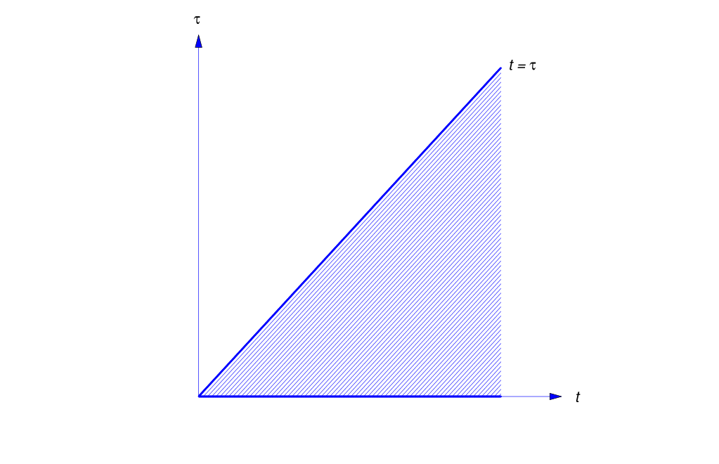
This iterated integral equals a double integral over the region shown in Figure 8.6.1. Reversing the order of integration yields
However, the substitution \(x=t-\tau\) shows that
Substituting this into (8.6.6) and noting that \(G(s)\) is independent of \(\tau\) yields
Example 8.6.1
Let
Verify that \({\cal L}(f\ast g)={\cal L}(f){\cal L}(g)\), as implied by the convolution theorem.
Solution We first compute
Since
it follows that
A Formula for the Solution of an Initial Value Problem
The convolution theorem provides a formula for the solution of an initial value problem for a linear constant coefficient second order equation with an unspecified. The next three examples illustrate this.
Example 8.6.2
Find a formula for the solution of the initial value problem
Solution Taking Laplace transforms in (8.6.7) yields
Therefore
From the table of Laplace transforms,
Since
the convolution theorem implies that
Therefore the solution of (8.6.7) is
Example 8.6.3
Find a formula for the solution of the initial value problem
Solution Taking Laplace transforms in (8.6.8) yields
Therefore
From the table of Laplace transforms,
Since
the convolution theorem implies that
Therefore the solution of (8.6.8) is
Example 8.6.4
Find a formula for the solution of the initial value problem
Solution Taking Laplace transforms in (8.6.9) yields
Therefore
From the table of Laplace transforms,
Since
the convolution theorem implies that
Therefore the solution of (8.6.9) is
Evaluating Convolution Integrals
We’ll say that an integral of the form \(\int_0^t u(\tau)v(t-\tau)\,d\tau\) is a convolution integral. The convolution theorem provides a convenient way to evaluate convolution integrals.
Example 8.6.5
Evaluate the convolution integral
Solution We could evaluate this integral by expanding \((t-\tau)^5\) in powers of \(\tau\) and then integrating. However, the convolution theorem provides an easier way. The integral is the convolution of \(f(t)=t^5\) and \(g(t)=t^7\). Since
the convolution theorem implies that
where we have written the second equality because
Hence,
Example 8.6.6
Use the convolution theorem and a partial fraction expansion to evaluate the convolution integral
Solution Since
the convolution theorem implies that
Expanding this in a partial fraction expansion yields
Therefore
Volterra Integral Equations
An equation of the form
is a Volterra integral equation. Here \(f\) and \(k\) are given functions and \(y\) is unknown. Since the integral on the right is a convolution integral, the convolution theorem provides a convenient formula for solving (8.6.11). Taking Laplace transforms in (8.6.11) yields
and solving this for \(Y(s)\) yields
We then obtain the solution of (8.6.11) as \(y={\cal L}^{-1}(Y)\).
Example 8.6.7
Solve the integral equation
Solution Taking Laplace transforms in (8.6.12) yields
and solving this for \(Y(s)\) yields
Hence,
Transfer Functions
The next theorem presents a formula for the solution of the general initial value problem
where we assume for simplicity that \(f\) is continuous on \([0,\infty)\) and that \({\cal L}(f)\) exists. In Exercises 11–14 it’s shown that the formula is valid under much weaker conditions on \(f\).
Theorem 8.6.3
Suppose \(f\) is continuous on \([0,\infty)\) and has a Laplace transform\(.\) Then the solution of the initial value problem
is
where \(y_1\) and \(y_2\) satisfy
and
and
Proof Taking Laplace transforms in (8.6.13) yields
where
Hence,
with
and
Taking Laplace transforms in (8.6.15) and (8.6.16) shows that
Therefore
and
Hence, (8.6.20) can be rewritten as
Substituting this into (8.6.18) yields
Taking inverse transforms and invoking the convolution theorem yields (8.6.14). Finally, (8.6.19) and (8.6.21) imply (8.6.17).∎
It is useful to note from (8.6.14) that \(y\) is of the form
where
depends on the initial conditions and is independent of the forcing function, while
depends on the forcing function and is independent of the initial conditions. If the zeros of the characteristic polynomial
of the complementary equation have negative real parts, then \(y_1\) and \(y_2\) both approach zero as \(t\to\infty\), so \(\lim_{t\to\infty}v(t)=0\) for any choice of initial conditions. Moreover, the value of \(h(t)\) is essentially independent of the values of \(f(t-\tau)\) for large \(\tau\), since \(\lim_{\tau\to\infty}w(\tau)=0\). In this case we say that \(v\) and \(h\) are transient and steady state components, respectively, of the solution \(y\) of (8.6.13). These definitions apply to the initial value problem of Example 8.6.4, where the zeros of
are \(-1\pm i\). From (8.6.10), we see that the solution of the general initial value problem of Example 8.6.4 is \(y=v+h\), where
is the transient component of the solution and
is the steady state component. The definitions don’t apply to the initial value problems considered in Examples 8.6.2 and 8.6.3, since the zeros of the characteristic polynomials in these two examples don’t have negative real parts.
In physical applications where the input \(f\) and the output \(y\) of a device are related by (8.6.13), the zeros of the characteristic polynomial usually do have negative real parts. Then \(W={\cal L}(w)\) is called the transfer function of the device. Since
we see that
is the ratio of the transform of the steady state output to the transform of the input.
Because of the form of
\(w\) is sometimes called the weighting function of the device, since it assigns weights to past values of the input \(f\). It is also called the impulse response of the device, for reasons discussed in the next section.
Formula (8.6.14) is given in more detail in Exercises 8–10 for the three possible cases where the zeros of \(p(s)\) are real and distinct, real and repeated, or complex conjugates, respectively.
8.6 Exercises
-
Express the inverse transform as an integral.
(a) \(\dst{1\over s^2(s^2+4)}\) (b) \(\dst{s\over(s+2)(s^2+9)}\) (c) \(\dst{s\over(s^2+4)(s^2+9)}\) (d) \(\dst{s\over(s^2+1)^2}\) (e) \(\dst{1\over s(s-a)}\) (f) \(\dst{1\over(s+1)(s^2+2s+2)}\) (g) \(\dst{1\over (s+1)^2(s^2+4s+5)}\) (h) \(\dst{1\over(s-1)^3(s+2)^2}\) (i) \(\dst{s-1\over s^2(s^2-2s+2)}\) (j) \(\dst{s(s+3)\over(s^2+4)(s^2+6s+10)}\) (k) \(\dst{1\over(s-3)^5s^6}\) (l) \(\dst{1\over(s-1)^3(s^2+4)}\) (m) \(\dst{1\over s^2(s-2)^3}\) (n) \(\dst{1\over s^7(s-2)^6}\)
Show answer
(a) \(\dst{{1\over 2}\int_0^t\tau\sin 2(t-\tau)\, d\tau}\) (b) \(\dst{\int_0^t e^{-2\tau}\cos 3(t-\tau)\,d\tau}\)
(c) \(\dst{{1\over 2}\int_0^t\sin 2\tau \cos 3(t-\tau)\,d\tau\mbox{ or } {1\over 3}\int_0^t\sin 3\tau \cos 2 (t-\tau)\,d\tau}\) (d) \(\dst{\int_0^t\cos\tau\sin (t-\tau)\, d\tau}\)
(e) \(\dst{\int_0^t e^{a\tau}d\tau}\) (f) \(\dst{e^{-t}\int_0^t\sin (t-\tau)\,d\tau}\) (g) \(\dst{e^{-2t}\int_0^t\tau e^\tau\sin (t-\tau)\,d\tau}\)
(h) \(\dst{{e^{-2t}\over 2}\int_0^t\tau^2 (t-\tau)e^{3\tau}\,d\tau}\) (i) \(\dst{\int_0^t (t-\tau)e^\tau\cos\tau\,d\tau}\) (j) \(\dst{\int_0^t e^{-3\tau}\cos\tau\cos 2 (t-\tau)\,d\tau}\)
(k) \(\dst{{1\over 4!5!}\int_0^t\tau^4 (t-\tau)^5 e^{3\tau}\,d\tau}\) (l) \(\dst{{1\over 4}\int_0^t\tau^2 e^\tau \sin 2(t-\tau)\,d\tau}\)
(m) \(\dst{{1\over 2}\int_0^t\tau(t-\tau)^2 e^{2(t-\tau)}\,d\tau}\) (n) \(\dst{{1\over 5!6!}\int_0^t (t-\tau)^5 e^{2(t-\tau)}\tau^6\,d\tau}\)
-
Find the Laplace transform.
(a) \(\dst{\int_0^t\sin a\tau\cos b(t-\tau)\, d\tau}\) (b) \(\dst{\int_0^t e^\tau\sin a(t-\tau)\,d\tau}\) (c) \(\dst{\int_0^t\sinh a\tau\cosh a(t-\tau)\,d\tau}\) (d) \(\dst{\int_0^t\tau(t-\tau)\sin \omega\tau\cos\omega (t-\tau)\,d\tau}\) (e) \(\dst{e^t\int_0^t\sin\omega\tau \cos\omega (t-\tau)\,d\tau}\) (f) \(\dst{e^t\int_0^t\tau^2 (t-\tau)e^\tau\,d\tau}\) (g) \(\dst{e^{-t}\int_0^t e^{-\tau}\tau\cos\omega (t-\tau)\,d\tau}\) (h) \(\dst{e^t\int_0^t e^{2\tau}\sinh (t-\tau)\,d\tau}\) (i) \(\dst{\int_0^t\tau e^{2\tau}\sin 2(t-\tau)\,d\tau}\) (j) \(\dst{\int_0^t (t-\tau)^3 e^\tau\, d\tau}\) (k) \(\dst{\int_0^t\tau^6 e^{-(t-\tau)}\sin 3(t-\tau)\,d\tau}\) (l) \(\dst{\int_0^t\tau^2 (t-\tau)^3\, d\tau}\) (m) \(\dst{\int_0^t (t-\tau)^7 e^{-\tau} \sin 2\tau\,d\tau}\) (n) \(\dst{\int_0^t (t-\tau)^4\sin 2\tau\,d\tau}\)
Show answer
(a) \(\dst{as\over(s^2+a^2)(s^2+b^2)}\) (b) \(\dst{a\over(s-1)(s^2+a^2)}\) (c) \(\dst{as\over(s^2-a^2)^2}\) (d) \(\dst{2\omega s(s^2-\omega^2)\over (s^2+\omega^2)^4}\)
(e) \(\dst{(s-1)\omega\over\left((s-1)^2+ \omega^2\right)^2}\) (f) \(\dst{2\over(s-2)^3 (s-1)^2}\) (g) \(\dst{s+1\over(s+2)^2\left[(s+1)^2+ \omega^2\right]}\)
(h) \(\dst{1\over(s-3)\left((s-1)^2-1\right)}\) (i) \(\dst{2\over(s-2)^2(s^2+4)}\) (j) \(\dst{6\over s^4(s-1)}\) (k) \(\dst{{3\cdot 6!\over s^7\left[(s+1)^2+ 9\right]}}\)
(l) \(\dst{12\over s^7}\) (m) \(\dst{{2\cdot 7!\over s^8\left[(s+1)^2+ 4\right]}}\) (n) \(\dst{48\over s^5(s^2+4)}\)
-
Find a formula for the solution of the initial value problem.
(a) \(y''+3y'+y=f(t),\quad y(0)=0,\quad y'(0)=0\)
(b) \(y''+4y=f(t),\quad y(0)=0,\quad y'(0)=0\)
(c) \(y''+2y'+y=f(t),\quad y(0)=0,\quad y'(0)=0\)
(d) \(y''+k^2y=f(t),\quad y(0)=1,\quad y'(0)=-1\)
(e) \(y''+6y'+9y=f(t),\quad y(0)=0,\quad y'(0)=-2\)
(f) \(y''-4y=f(t),\quad y(0)=0,\quad y'(0)=3\)
(g) \(y''-5y'+6y=f(t),\quad y(0)=1,\quad y'(0)=3\)
(h) \(y''+\omega^2y=f(t),\quad y(0)=k_0,\quad y'(0)=k_1\)
Show answer
(a) \(\dst{y={2\over\sqrt{5}}\int_0^t f(t-\tau)e^{-3\tau/2}\sinh{\sqrt{5}\tau\over 2}\,d\tau}\) (b) \(\dst{y={1\over2}\int_0^t f(t-\tau)\sin 2\tau\,d\tau}\)
(c) \(\dst{y=\int_0^t\tau e^{-\tau}f(t-\tau)\; d\tau}\) (d) \(\dst{y(t)=-{1\over k}\sin kt +\cos kt+ {1\over k}\int_0^t f(t-\tau)\sin k\tau\,d\tau}\)
(e) \(\dst{y=-2te^{-3t}+\int_0^t\tau e^{-3\tau}f(t-\tau)\,d\tau}\) (f) \(\dst{y={3\over 2}\sinh 2t+{1\over 2}\int_0^t f(t-\tau)\sinh 2\tau\,d\tau}\)
(g) \(\dst{y=e^{3t}+\int_0^t(e^{3\tau} -e^{2\tau})f(t-\tau)\,d\tau}\) (h) \(\dst{y={k_1\over\omega} \sin\omega t+k_0\cos\omega t+{1\over\omega}\int_0^t f(t-\tau)\sin \omega\tau\,d\tau}\)
-
Solve the integral equation.
(a) \(\dst{y(t)=t-\int_0^t (t-\tau) y(\tau)\,d\tau}\)
(b) \(\dst{y(t)=\sin t-2 \int_0^t\cos (t-\tau) y (\tau)\,d\tau}\)
(c) \(\dst{y(t)=1+2 \int_0^ty(\tau)\cos(t-\tau)\,d\tau}\) (d) \(\dst{y(t)=t+\int_0^t y(\tau)e^{-(t-\tau)}\,d\tau}\) (e) \(\dst{y'(t)=t+\int_0^t y(\tau)\cos (t-\tau)\,d\tau,\, y(0)=4}\)
(f) \(\dst{y(t)=\cos t-\sin t+ \int_0^t y(\tau)\sin (t-\tau)\,d\tau}\)
[2]
Show answer
(a) \(y=\sin t\)(b) \(y=te^{-t}\) (c) \(y=1+2te^t\) (d) \(\dst{y=t+{t^2\over 2}}\)
(e) \(\dst{y=4+{5\over 2}t^2+{1\over 24}t^4}\) (f) \(\dst{y=1-t}\)
-
Use the convolution theorem to evaluate the integral.
(a) \(\dst{\int_0^t (t-\tau)^7\tau^8\, d\tau}\) (b) \(\dst{\int_0^t(t-\tau)^{13}\tau^7\,d\tau}\) (c) \(\dst{\int_0^t(t-\tau)^6\tau^7\, d\tau}\) (d) \(\dst{\int_0^te^{-\tau}\sin(t-\tau)\,d\tau}\) (e) \(\dst{\int_0^t\sin\tau\cos2(t-\tau)\,d\tau}\)
[2]
Show answer
(a) \(\dst{7!8!\over 16!}t^{16}\) (b) \(\dst{13!7!\over 21!} t^{21}\) (c) \(\dst{6!7!\over 14!}t^{14}\) (d) \(\dst{1\over2}(e^{-t}+\sin t-\cos t)\) (e) \(\dst{1\over3}(\cos t-\cos 2t)\)
-
Show that
\[ \int_0^tf(t-\tau)g(\tau)\,d\tau=\int_0^tf(\tau)g(t-\tau)\,d\tau \]by introducing the new variable of integration \(x=t-\tau\) in the first integral.
-
Use the convolution theorem to show that if \(f(t)\leftrightarrow F(s)\) then
\[ \int_0^tf(\tau)\,d\tau\leftrightarrow {F(s)\over s}. \] -
Show that if \(p(s)=as^2+bs+c\) has distinct real zeros \(r_1\) and \(r_2\) then the solution of
\[ ay''+by'+cy=f(t),\quad y(0)=k_0,\quad y'(0)=k_1 \]is
\begin{eqnarray*} y(t)&=&\; k_0{r_2e^{r_1t}-r_1e^{r_2t}\over r_2-r_1}+k_1{e^{r_2t}-e^{r_1t} \over r_2-r_1} \\ &&+{1\over a(r_2-r_1)}\int_0^t(e^{r_2\tau}-e^{r_1\tau})f(t-\tau)\,d\tau. \end{eqnarray*} -
Show that if \(p(s)=as^2+bs+c\) has a repeated real zero \(r_1\) then the solution of
\[ ay''+by'+cy=f(t),\quad y(0)=k_0,\quad y'(0)=k_1 \]is
\[ y(t)=\; k_0(1-r_1t)e^{r_1t}+k_1te^{r_1t} +{1\over a}\int_0^t\tau e^{r_1\tau}f(t-\tau)\,d\tau. \] -
Show that if \(p(s)=as^2+bs+c\) has complex conjugate zeros \(\lambda\pm i\omega\) then the solution of
\[ ay''+by'+cy=f(t),\quad y(0)=k_0,\quad y'(0)=k_1 \]is
\begin{eqnarray*} y(t)&=&\; e^{\lambda t}\left[k_0(\cos\omega t-{\lambda\over\omega}\sin\omega t)+{k_1\over\omega}\sin\omega t\right] \\ &&+{1\over a\omega}\int_0^te^{\lambda t}f(t-\tau)\sin\omega\tau\, d\tau. \end{eqnarray*} -
Let
\[ w={\cal L}^{-1}\left(1\over as^2+bs+c\right), \]where \(a,b\), and \(c\) are constants and \(a\ne0\).
Show that \(w\) is the solution of
\[ aw''+bw'+cw=0,\quad w(0)=0,\quad w'(0)={1\over a}. \]Let \(f\) be continuous on \([0,\infty)\) and define
\[ h(t)=\int_0^t w(t-\tau)f(\tau)\,d\tau. \]Use Leibniz’s rule for differentiating an integral with respect to a parameter to show that \(h\) is the solution of
\[ ah''+bh'+ch=f,\quad h(0)=0,\quad h'(0)=0. \]Show that the function \(y\) in Eqn. (8.6.14) is the solution of Eqn. (8.6.13) provided that \(f\) is continuous on \([0,\infty)\); thus, it’s not necessary to assume that \(f\) has a Laplace transform.
-
Consider the initial value problem
\[ ay''+by'+cy=f(t),\quad y(0)=0,\quad y'(0)=0, \tag*{\rm (A)} \]where \(a,b\), and \(c\) are constants, \(a\ne0\), and
\[ f(t)=\left\{\begin{array}{cc}f_0(t),&0\le t<t_1,\\[5pt] f_1(t),&t\ge t_1.\end{array}\right. \]Assume that \(f_0\) is continuous and of exponential order on \([0,\infty)\) and \(f_1\) is continuous and of exponential order on \([t_1,\infty)\). Let
\[ p(s)=as^2+bs+c. \]Show that the Laplace transform of the solution of (A) is
\[ Y(s)={F_0(s)+e^{-st_1}G(s)\over p(s)} \]where \(g(t)=f_1(t+t_1)-f_0(t+t_1)\).
Let \(w\) be as in Exercise 11. Use Theorem 8.4.2 and the convolution theorem to show that the solution of (A) is
\[ y(t)=\int_0^t w(t-\tau)f_0(\tau)\,d\tau+u(t-t_1)\int_0^{t-t_1} w(t-t_1-\tau)g(\tau)\,d\tau \]for \(t>0\).
Henceforth, assume only that \(f_0\) is continuous on \([0,\infty)\) and \(f_1\) is continuous on \([t_1,\infty)\). Use Exercise 11 (a) and (b) to show that
\[ y'(t)=\int_0^t w'(t-\tau)f_0(\tau)\,d\tau+u(t-t_1)\int_0^{t-t_1} w'(t-t_1-\tau)g(\tau)\,d\tau \]for \(t>0\), and
\[ y''(t)={f(t)\over a}+\int_0^t w''(t-\tau)f_0(\tau)\,d\tau+u(t-t_1)\int_0^{t-t_1} w''(t-t_1-\tau)g(\tau)\,d\tau \]for \(0<t<t_1\) and \(t>t_1\). Also, show \(y\) satisfies the differential equation in (A) on\((0,t_1)\) and \((t_1,\infty)\).
Show that \(y\) and \(y'\) are continuous on \([0,\infty)\).
-
Suppose
\[ f(t)=\left\{\begin{array}{cl} f_0(t),&0\le t < t_1,\\[5pt] f_1(t),&t_1\le t < t_2,\\ &\vdots\\ f_{k-1}(t),&t_{k-1}\le t < t_k,\\[5pt] f_k(t),&t\ge t_k, \end{array}\right. \]where \(f_m\) is continuous on \([t_m,\infty)\) for \(m=0,\dots,k\) (let \(t_0=0\)), and define
\[ g_m(t)=f_m(t+t_m)-f_{m-1}(t+t_m) ,\, m=1,\dots,k. \]Extend the results of Exercise 12 to show that the solution of
\[ ay''+by'+cy=f(t),\quad y(0)=0,\quad y'(0)=0 \]is
\[ y(t)=\int_0^t w(t-\tau)f_0(\tau)\,d\tau+\sum_{m=1}^ku(t-t_m) \int_0^{t-t_m}w(t-t_m-\tau)g_m(\tau)\,d\tau. \] -
Let \(\{t_m\}_{m=0}^\infty\) be a sequence of points such that \(t_0=0\), \(t_{m+1}>t_m\), and \(\lim_{m\to\infty}t_m=\infty\). For each nonegative integer \(m\) let \(f_m\) be continuous on \([t_m,\infty)\), and let \(f\) be defined on \([0,\infty)\) by
\[ f(t)=f_m(t),\quad t_m\le t<t_{m+1}\quad m=0,1,2\dots. \]Let
\[ g_m(t)=f_m(t+t_m)-f_{m-1}(t+t_m),\quad m=1,\dots,k. \]Extend the results of Exercise 13 to show that the solution of
\[ ay''+by'+cy=f(t),\quad y(0)=0,\quad y'(0)=0 \]is
\[ y(t)=\int_0^t w(t-\tau)f_0(\tau)\,d\tau+\sum_{m=1}^\infty u(t-t_m) \int_0^{t-t_m}w(t-t_m-\tau)g_m(\tau) \,d\tau. \]Hint: See Exercise30.